Will there be presentation slides in future classes, or is everything embedded into the quarto/html files for all lectures?
The material will primarily be in quarto/html files and not slides.
Specifics of what topics will be covered exactly. * I don’t have a list of all the specific functions we will be covering, but you are welcome to peruse the BSTA 504 webpage from Winter 2023 to get more details on topics we will be covering. We will be closely following the same class materials.
Identifying which section of the code we were discussing during the lecture
Thanks for letting me know. I will try to be clearer in the future, and also jump around less. Please let me know in class if you’re not sure where we are at.
The material covered towards the end of the class felt a bit difficult to keep up with. I wish we would have been told to read the materials from Week 1 (or at least skim them) ahead of Day 1, because I quickly lost track of the conversation when shortcuts were used super quickly, for example, or when we jumped from chunks of code to another topic without reflecting on them. I still had 70% of the material down and I wrote great notes during the discussion (which I later filled in with the script that was on the class website), but I think it the beginner/intermediate programming lingo that was used to explain ideas here confused me at times. Thus, I struggled to keep up with discussions around packages / best coding practices, especially when they were not mentioned directly on the script (where I could follow along!).
Thanks for the feedback. In future years, we will reach out to students before the term to let them know about the readings to prepare for class. Please let us know if there is lingo we are using that you are not familiar with. Learning R and coding is a whole new language!
RStudio
I have trouble thinking through where things are automatically downloaded, saved, and running from. I can attend office hours for this!
Office hours are always a great idea. I do recommend paying close attention to where files are being saved when downloading and preferably specifying their location instead using the default location. Having organized files will make working on complex analyses much easier.
How to read the course material in R. While it made sense in real time it may be difficult when going back over the material.
Getting used to reading code and navigating the rendered html files takes a while, and is a part of learning R. Figuring out how to take notes for yourself that works for you is also a learning curve. I recommend taking notes in the qmd files as we go through them in class. After class you can summarize and transfer key points to other file formats that you are more used to using. I personally have a folder in my Google drive filled with documents on different R programming topics. It started with one file, and then eventually expanded to multiple files on different topics in an attempt to organize my notes better. Whenever I learn something new (such as an R function or handy R package) that I want to keep for future reference, I add to them with links to relevant webpages and/or filenames and locations of where I used them.
Code
What does the pacman package do? I have it installed but I’m not sure what it is actually used for.
I didn’t go into pacman in Day 1. The p_load() function from the pacman package (usually run as pacman::p_load()) lets you load many packages at once without separately using the library() function for each individually.
An added bonus is that by default it will install packages you don’t already have, unless you specify install = FALSE.
Another option is to set update = TRUE so that it will automatically update packages. I do not use this option though since sometimes updating packages causes conflicts with other packages or older code.
You can read more about the different options in the documentation. This Medium article also has some tips on using pacman.
The part on when to load in packages once they’ve already been loaded in - like for example would it be good to put that as a step in our homework 1 .qmd at the top? Or not necessary since they’re already loaded in to R Studio from the work we did in class yesterday? What would happen if we try to load them in and they were already loaded in, would the .qmd file not render and show an error?
I always load my packages at the very top of the .qmd files, usually in the first code chunk (with the setup label). If you still have a previous R session open, then yes you don’t need to load the packages again to run code within RStudio. However, when a file is rendered it starts with an empty workspace, which is why our qmd file must include code that loads the packages (either using library() or pacman::p_load(). We don’t have to load packages at the beginning of the file, just before we have code that depends on the packages being used.
I didn’t understand the part where we talked about num, char, logical combinations (line 503).
The content of the objects char_logical, num_char, num_logical, and tricky were designed specifically to be confusing and thus make us aware of how R will decide to assign the data type when a vector is a mix of data types. Some key takeaways are below. Let me know if you sitll have questions about this.
Numbers and logical/boolean (TRUE, FALSE) do not have double quotes around them, but character strings do. If you add double quotes to a number or logical, then R will treat it as a character string.
If a vector is a mix of numbers and character strings, then the data type of the vector is character.
If a vector is a mix of numbers and logical, then the data type of the vector is numeric and the logical value is converted to a numeric value (TRUE=1, FALSE=0).
If a vector is a mix of character strings and logical, then the data type of the vector is character and the logical value is converted to a character string and no longer operates as a logical (i.e. no longer equal to 1 or 0).
Lines 614-619, confused what the ratio means there. Could you go over the correct code (or options of the correct code) for challenge 5?
The code 1:4 or 6:9 creates sequences of integers starting with the first specified digit and ending at the last specified digit. For example, 1:4 is the vector with the digits 1 2 3 4. You can also create decreasing sequences by making the first number the bigger one. For example, 9:7 is the vector 9 8 7.
Challenge 5:
more_heights_complete <- na.omit(more_heights)
median(more_heights_complete)
You could also get the median of more_heights without first removing the missing values with median(more_heights, na.rm = TRUE).
how to count the TRUE values in a logical vector
TRUE is equal to 1 in R (and FALSE is equal to 0), and the function sum() adds up the values in a vector. Thus, sum(TRUE, FALSE, TRUE) is equal to 2. Similarly, sum(TRUE, FALSE, 5) is equal to 6.
The way I used it in class though is by counting how many values in the vector z (which was 7 9 11 13) are equal to 9. To do that I used the code sum(z == 9). Breaking that down, the code inside the parentheses z == 9 is equal to FALSE TRUE FALSE FALSE since the == means “equals to” in R.
You can read up more on boolean and logical operators at the R-bloggers post.
Clearest Points
Thank you for the feedback!
Class logistics
Syllabus/course structure
The syllabus review.
Overall expectations and course flow
Introduction to the class (first half of the class); conversation around syllabus; and the Quarto introduction
Quarto
How to create and edit a Quarto document in RStudio.
The differences between quarto and markdown
rmarkdown is no more, quarto it is!
Coding
Having code missing and fixing it in front of the class was helpful in troubleshooting.
Just running through all the commands was very clear and easy to follow
Basic R set up for quarto and introduction to R objects, vectors, etc.
Introduction, functions, and explanations was the clearest for me.
Classification of the objects in logical, character, and numeric
Not necessarily a point, but I really liked when we were encouraged to use the shortcut keys for various commands on R and other little things like switching code between console vs inline , I have used R before for a class briefly but I never knew all these ways by which I can save time and be efficient while writing a code.
Week 2
Muddiest points
When discussing untidy data, the difference between long data and wide data was unclear.
We’ll be discussing the difference between long and wide data in more detail later in the course when we convert a dataset between the two. For now, you can take a look at an example I created for our BERD R workshops. The wide data in that example are not “tidy” since each cell contains two pieces of information: both the SBP and the visit number. In contrast, the long data have a separate column indicating which visit number the data in a given row are from.
for the “summary()” function, is there a way to summarize all but one variable in a dataset?
Yes! I sometimes restrict a dataset to a couple of variables for which I want to see the summary. I usually use the select() function for this, which we will be covering later in the course. For now, you can take a look at some select() examples from the BERD R workshops (see slides 29-32).
Differences between a tibble and a data.frame
I’m not surprised to see this show up as a muddiest point! Depending on your level of experience with R, at this point in the class some of the differences are difficult to explain since we haven’t done much coding yet. The tibble vignette lists some of the differences though if you are interested. For our purposes, they are almost the same thing. When some differences come up later in the course, I will point them out.
Clearest Points
Thanks for the feedback!
I enjoyed going through the code and viewing the functions. I haven’t really used skimr before and that was nice to see.
I like using skmir, but have recently been using get_summary_stats() from the rstatix package when teaching. It is only for numeric variables though. See a get_summary_stats() example from my BSTA 511 class.
Loading data.
How to load data into R was clearest.
Good to know that loading data was clear. This part can be tricky sometimes!
ggplot
Hopefully this will still be clear when we cover more advanced options in ggplot!
Week 3
Muddiest points
here package
The here package takes a bit to explaining, but, compared to the old way of doing things, it is a real life saver. The issue in the past had to do with relative file paths, especially with .qmd files that are saved in sub-folders. The .qmd file recognizes where it is saved as the root file path, which is okay with a one-off .qmd file. But when working in projects (recommended) and striving for reproducible R code (highly recommended), the here package save a lot of headache.
Project-oriented workflows are recommended. Here package solves some old headaches. It gets easier with practice.
Question about using here
… how [here] can be used in certain instances where one may not remember if they switched to a new qmd file? In that case, would you suggest to use the “here” command each time you work on a project where there’s a chance that you’ll switch between qmd files and would like to use the same data file throughout? Is there any other way to better use this function or tips on how you deal with it?
There is a difference between working interactively in RStudio where data are loaded to the Environment. In this case, loading a data set once means that it can be used in any other code while working in the environment.
Issues will com up when you go to render a .qmd that doesn’t have the data loaded within that .qmd. It won’t look to the environment for the data; it looks to the filepath that you specify in the .qmd. Best practice is to write the code to load the data in each .qmd or .R script so that R knows where to look for the data that you want it to operate on / analyze.
The ! function. It seems like sometimes we use ! and sometimes we use -. Are they interchangeable, or each with different types of functions?
! – the exclamation point can be read as “not” it is primarily used in logical statements
- – the minus sign can be used in more instances
to do actual arithmetic (i.e. subtraction)
to indicate a negative number
with dplyr::select() to remove or not select a column, or exclusion
# Subtraction5-3
[1] 2
# Negationx <-10-x
[1] -10
# Selection/exclusionlibrary(dplyr)
Attaching package: 'dplyr'
The following objects are masked from 'package:stats':

    filter, lag
The following objects are masked from 'package:base':

    intersect, setdiff, setequal, union
We didn’t cover it in the lecture notes, but then it appeared in the example. I suggest to read/work through the fill vignette; the examples there are good ones to show what the function does. Then look back a the smoke_messy data set in Part 3 and think about why this command would be useful to clean up the data and for filling in missing values.
Loading data into R
It gets easier and hopefully you get to see more example in the notes and practice with the homework. This tutorial is pretty good. So is the readxl vignette and the readr vignette.
Reasonable width, height, and dpi values when using ggsave
This takes some trial and error and depends on the purpose. For draft figures, dpi = 70 might be okay, but a journal might require dpi above 300 for publication. In Quarto, rendering an html, the figure defaults are 7x5 inches (Link). We talked about in class how you can use the plot panes to size your figures by trial and error.
For more info and learning about tidyselect, please run this code in your console:
# install remotes packageinstall.packages("remotes")# use remotes to install this package from githubremotes::install_github("laderast/tidyowl")# load tidyowl packagelibrary(tidyowl)# interactive tutorialtidyowl::learn_tidyselect()
Here is also a link with a list of the selectors and links to each one. For example, there is a link to starts_with and a bunch of examples.
In office hours, someone didn’t know about this fact and wanted to make sure everyone knows about it.
Important keyboard shortcut
In RStudio the keyboard shortcut for the pipe operator %>% (or native pipe |>) is Ctrl + Shift + M (Windows) or Cmd + Shift + M (Mac).
Note: Ctrl + Shift + M also works on a Mac.
The difference between NA value and 0
NA (Not Available)
NA is a special value in R that represents missing or undefined data.
0 is a numeric value representing the number zero. It is a valid and well-defined numerical value in R.
It’s important to handle NA values appropriately in data analysis and to consider their impact on calculations, as operations involving NA may result in NA.
NA+5# The result is NA
[1] NA
0+5# The results is 5
[1] 5
x <-c(1, 2, NA, 4)sum(x) # The result is NA
[1] NA
# Using the argument na.rm = TRUE, means to ignore the NAssum(x, na.rm =TRUE) # The results is 7
[1] 7
x <-c(1, 2, 0, 4)sum(x) # The result is 7
[1] 7
across() and it’s usage
The biggest advantage that across brings is the ability to perform the same data manipulation task to multiple columns.
Below the values in three columns are all set to the mean value using the mean(). I had to write out the function and the variable names three times.
We’ve seen the ~ and .x used with dplyr::across(). We will see them again later when we get to the package purrr.
In the tidyverse, ~ and .x are used to create what they call lambda functions which are part of the purrr syntax. We have not talked about functions yet, but purrr package and the dplyr::across() function allow you to specify functions to apply in a few different ways:
Above, just using the function name, we are not able to provide the additional argument na.rm = TRUE to the mean() function, so the columns are now all NA values because there were missing (NA) values in those columns.
An anonymous function, e.g. \(x) x + 1 or function(x) x + 1.
This has not been covered yet. R lets you specify your own functions and there are two basic ways to do it.
Now we are able to use the additional argument na.rm = TRUE and the columns are now the means of the valid values in those columns.
A purrr-style lambda function, e.g. ~ mean(.x, na.rm = TRUE)
We use ~ to indicate that we are supplying a lambda function and we use .x as a placeholder for the argument within our lambda function to indicate where to use the variable.
Some of these are purrr focused which we have not covered yet. Others use dplyr::across() withing the dplyr::summarize() function which we will be covering soon
For compatibility with the classic interface, can also be a formula or character vector. Use either a one sided formula, ~a + b, or a character vector, c("a", "b").
Here it is being used to specify a formula.
Though per the vignette, the vars() function is preferred syntax:
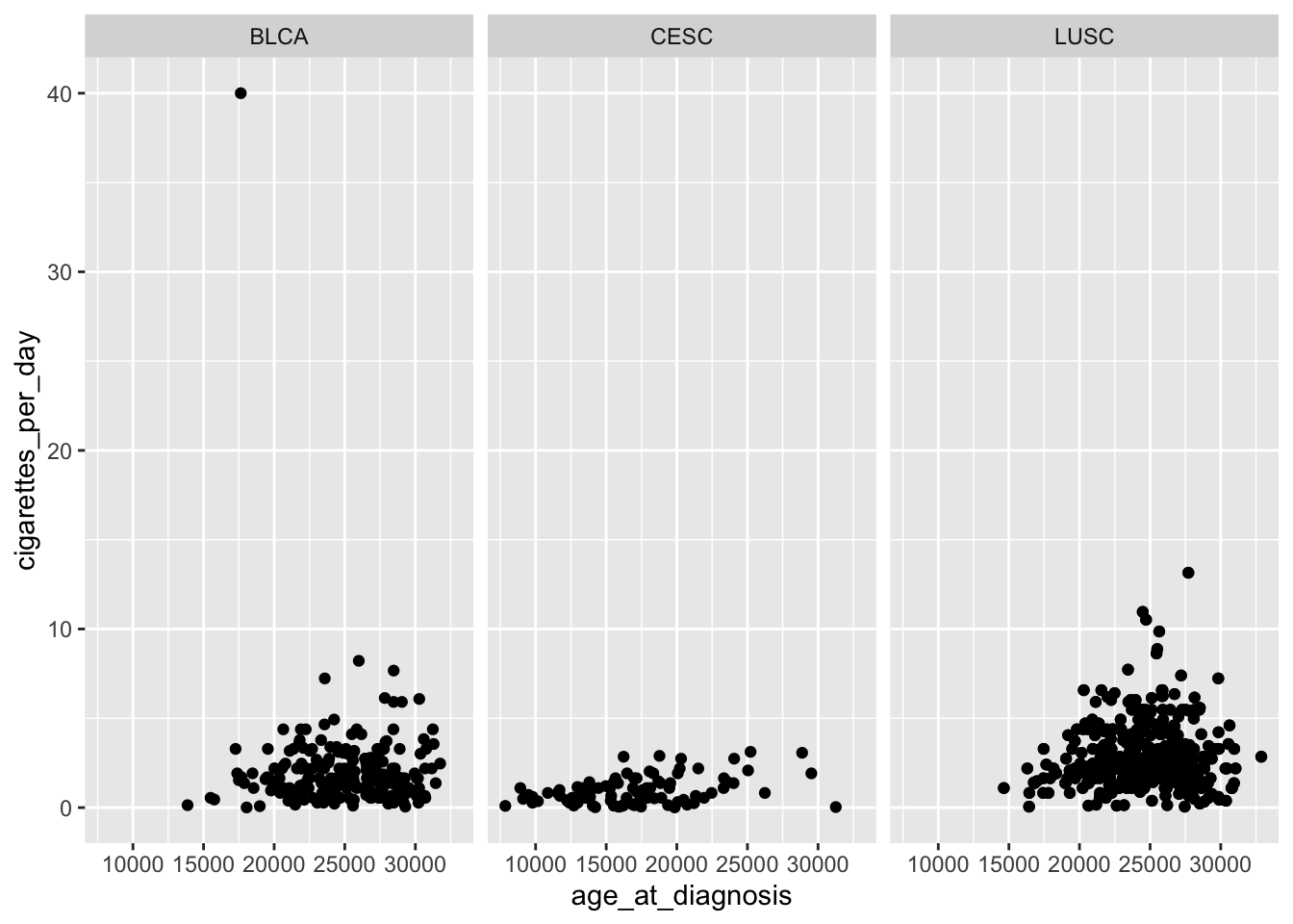
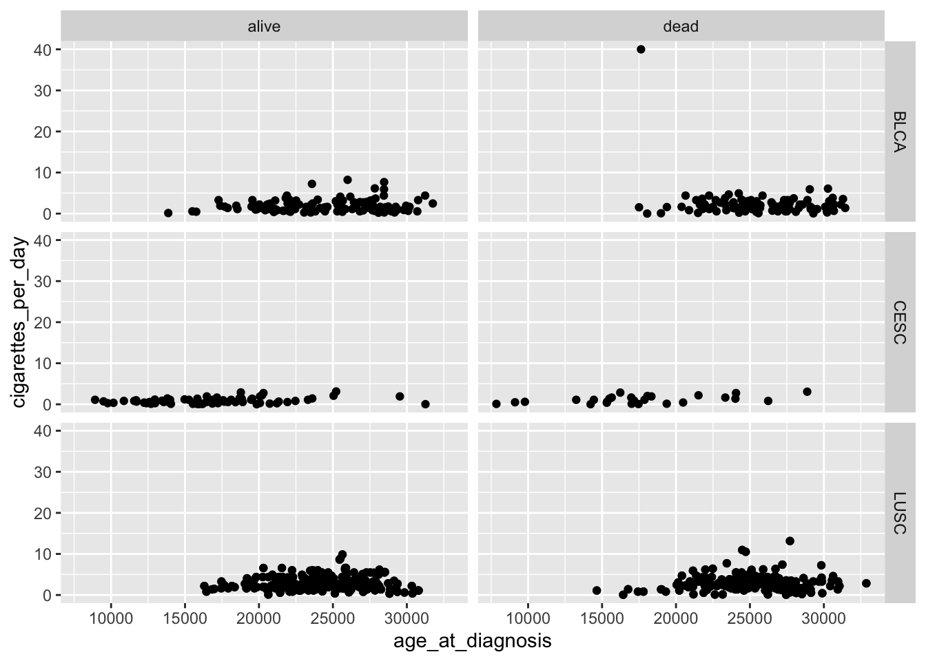
For compatibility with the classic interface, rows can also be a formula with the rows (of the tabular display) on the LHS and the columns (of the tabular display) on the RHS; the dot in the formula is used to indicate there should be no faceting on this dimension (either row or column).
Again, it is being used to specify a formula.
Though per the vignette, the ggplot2::vars() function with the arguments rows and cols seems to be preferred:
 cigarettes_category    n    percent
                 0-5 1100 0.95486111
                  6+   52 0.04513889
In this example, the column cigarettes_category is assigned the value “0-5” if cigarettes_per_day is less than 6 and “6+” otherwise.
case_when() function
case_when() is more versatile and is suitable for handling multiple conditions with multiple possible outcomes. It is essentially a vectorized form of a switch or if_else chain.
It allows you to specify multiple conditions and their corresponding values.
smoke_complete |>mutate(cigarettes_category =case_when( cigarettes_per_day <2~"0 to 2", cigarettes_per_day <4~"2 to 4", cigarettes_per_day <6~"4 to 6", cigarettes_per_day >=6~"6+" )) |>mutate(cigarettes_category =factor(cigarettes_category)) |> janitor::tabyl(cigarettes_category)
 cigarettes_category   n    percent
              0 to 2 455 0.39496528
              2 to 4 493 0.42795139
              4 to 6 152 0.13194444
                  6+  52 0.04513889
In this example, the column cigarettes_category is assigned the value “0 to 2” if cigarettes_per_day is less than 2, “2 to 4” if less than 4 (but greater than 2), “4 to 6” if less than 6 (but greater than 4), and “6+” otherwise.
Use if_else() when you have a simple binary condition, and use case_when() when you need to handle multiple conditions with different outcomes. case_when() is more flexible and expressive when dealing with complex conditional transformations.
The difference between a theme and and a palette.
In ggplot2, a theme and a palette serve different purposes and are used in different contexts. In summary, a theme controls the overall appearance of the plot, while a palette is specifically related to the colors used to represent different groups or levels within the data. Both themes and palettes contribute to visual appeal and readability of your plot.
Theme:
A theme in ggplot2 refers to the overall visual appearance of the plot. It includes elements such as fonts, colors, grid lines, background, and other visual attributes that define the look and feel of the entire plot.
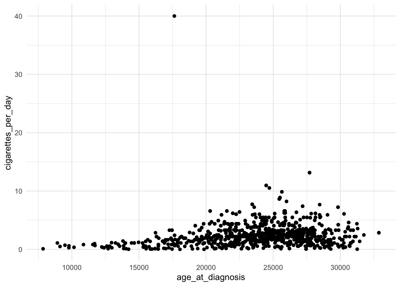
Themes are set using functions like theme_minimal(), theme_classic(), or custom themes created with the theme() function. Themes control the global appearance of the plot.
library(ggplot2)# Example using theme_minimal()ggplot(data = smoke_complete, aes(x = age_at_diagnosis, y = cigarettes_per_day)) +geom_point() +theme_minimal()
Palette:
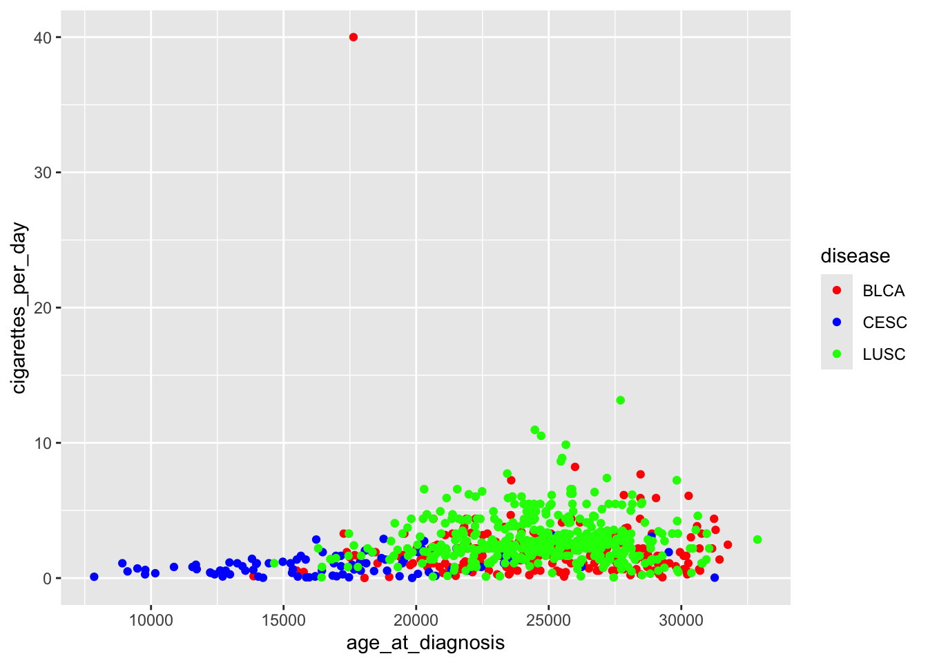
A palette, on the other hand, refers to a set of colors used to represent different levels or categories in the data. It is particularly relevant when working with categorical or discrete data where you want to distinguish between different groups.
Palettes are set using functions like scale_fill_manual() or scale_color_manual(). You can specify a vector of colors or use pre-defined palettes from packages like RColorBrewer or viridis (we looked at the viridis package in class).
# Example using a color paletteggplot(data = smoke_complete, aes(x = age_at_diagnosis, y = cigarettes_per_day, color = disease)) +geom_point() +scale_color_manual(values =c("red", "blue", "green"))
Be careful what you pipe to and from
An error came up where a data frame was being piped to a function that did not accept a data frame as an argument (it accepted a vector)
# starwars data frame was loaded earlier with the ggplot2 packagestarwars |> dplyr::n_distinct(species)
Error in list2(...): object 'species' not found
starwars is a data frame.
dplyr::n_distinct() only accepts a vector as an argument (check the help ?dplyr::n_distinct)
So we need to pipe a vector to the dplyr::n_distinct() function:
dplyr::select() accepts a data frame as its first argument and it return a vector (see the help ?dplyr::select) which we can then pipe to dplyr::n_distinct().
The %>% or |> takes the output of the expression on its left and passes it as the first argument to the function on its right. The class / type of output on the left needs to agree or be acceptable as the first argument to the function on the right.
This gets better with experience. You are all still very new to R so be patient with yourself.
How to organize all of the material to understand the structure of how the R language works, rather than to keep track of all of the commands in an anecdotal way.
Again, I think that this gets better with experience. Though the R language, being open source, a lot of syntax is package dependent. So you need to be careful that some of the syntax we use with dplyr and the tidyverse will be different in base R or in other packages. This is something that comes with open source software (compared to Stata or SAS). The good news is that learning to use packages sets you up to better learn newer (to you) packages down the road.
Week 5
case_when() vs ifelse()
The difference between case_when and ifelse
ifelse() is the base R version of tidyverse’s case_when()
I prefer using case_when() since it’s easier to follow the logic.
case_when() is especially useful when there are more than two logical conditions being used.
The example below creates a binary variable for bill length (long vs not long) using both case_when() and ifelse() as a comparison.
      species          island    bill_length_mm  bill_depth_mm
 Adelie   :152   Biscoe   :168   Min.   :32.10   Min.   :13.10
 Chinstrap: 68   Dream    :124   1st Qu.:39.23   1st Qu.:15.60
 Gentoo   :124   Torgersen: 52   Median :44.45   Median :17.30
                                 Mean   :43.92   Mean   :17.15
                                 3rd Qu.:48.50   3rd Qu.:18.70
                                 Max.   :59.60   Max.   :21.50
                                 NA's   :2       NA's   :2
 flipper_length_mm  body_mass_g       sex           year
 Min.   :172.0     Min.   :2700   female:165   Min.   :2007
 1st Qu.:190.0     1st Qu.:3550   male  :168   1st Qu.:2007
 Median :197.0     Median :4050   NA's  : 11   Median :2008
 Mean   :200.9     Mean   :4202                Mean   :2008
 3rd Qu.:213.0     3rd Qu.:4750                3rd Qu.:2009
 Max.   :231.0     Max.   :6300                Max.   :2009
 NA's   :2         NA's   :2
            long_bill4
 long_bill3       long medium short NA_
       long         57      0     0   0
     medium          0    185     0   2
      short          0      0   100   0
separate()
Different ways of using the function separate, it was a bit unclear that when to use one or the other or examples of my research data where it’ll be most relevant to use.
Choosing the “best” way of using separate() is overwhelming at first.
I recommend starting with the simplest use case with a string being specified in sep = " ":
separate(data, col, into, sep = " ")
Which of the various versions we showed to use depends on how the data being separated are structured.
Most of the time I have a simple character, such as a space (sep = " ") or a comma (sep = ",") that I want to separate by.
If the data are structured in a more complex way, then one of the stringr package options might come in handy.
here::here()
TSV files, very neat… But also, I got a bit confused when you did the render process around 22:00-23:00 minutes. Also, “here: and also”here” Directories/root directories. I was a bit confused about in what situations we would tangibly utilize this/if it is beneficial.
Great question! This is definitely not intuitive, which is why I wanted to demonstrate it in class.
The key is that
when rendering a qmd file the current working directory is the folder the file is sitting in,
while when running code in a file within RStudio the working directory is the folder where the .Rproj file is located.
This distinction is important when loading other files from our computer during our workflow, and why here::here() makes our workflow so much easier!
what functions will only work within another function (generally)
I’m not aware of functions that only work standalone within other functions. For example, the mean() function works on its own, but can also be used within a summarise().
      species          island    bill_length_mm  bill_depth_mm
 Adelie   :152   Biscoe   :168   Min.   :32.10   Min.   :13.10
 Chinstrap: 68   Dream    :124   1st Qu.:39.23   1st Qu.:15.60
 Gentoo   :124   Torgersen: 52   Median :44.45   Median :17.30
                                 Mean   :43.92   Mean   :17.15
                                 3rd Qu.:48.50   3rd Qu.:18.70
                                 Max.   :59.60   Max.   :21.50
                                 NA's   :2       NA's   :2
 flipper_length_mm  body_mass_g       sex           year
 Min.   :172.0     Min.   :2700   female:165   Min.   :2007
 1st Qu.:190.0     1st Qu.:3550   male  :168   1st Qu.:2007
 Median :197.0     Median :4050   NA's  : 11   Median :2008
 Mean   :200.9     Mean   :4202                Mean   :2008
 3rd Qu.:213.0     3rd Qu.:4750                3rd Qu.:2009
 Max.   :231.0     Max.   :6300                Max.   :2009
 NA's   :2         NA's   :2
  long_bill1         long_bill2         long_bill3         long_bill4
 Length:344         Length:344         Length:344         Length:344
 Class :character   Class :character   Class :character   Class :character
 Mode  :character   Mode  :character   Mode  :character   Mode  :character
# base Rmean(penguins$bill_length_mm, na.rm =TRUE)
[1] 43.92193
# with summarizepenguins %>%summarize(mean(bill_length_mm, na.rm =TRUE))
The .fns=list part of the across code is where we specify the function(s) that we want to apply to the specified columns.
Above we only specified one function (mean()), but we can specify additional functions as well, which is when we need to create a list to list all the functions we want to apply.
Below I apply the mean and standard deviation functions:
In general, lists are another type of R object to store information, whether data, lists of functions, output from regression models, etc. While concatenate is just a vector of values, lists are multidimensional. We will be learning more about lists in parts 7 and 8.
You can learn more about across() at its help file.
case_when() vs ifelse()
still a little confused on the difference between ifelse and casewhen, understand they are very similar but still confused on when it is best to use one over another
The two functions can be used interchangeably. * ifelse() is the original function from base R
case_when() is the user-friendly version of ifelse() from the dplyr package
I recommend using case_when(), and it is what I use almost exclusively in my own work. My guess is that ifelse() was included in the notes since you might run into the function when reading R code on the internet.
Just be careful that you preserve missing values when using case_when() as we discussed last time.
factor levels
working with factor levels doesn’t feel totally intuitive yet. I think that’s because I tend to get confused with anything involving a concatenated list.
Working with factor variables takes a while to get used to, and in particular with their factor levels.
We will be looking at more examples with factor variables in the part 6 notes. See sections 2.8 and 4.
You can think of a concatenated list(c(...)) as a vector of values or a column of a dataset. Concatenating lets us create a set of values, which we typically create to use for some other purpose, such as specifying the levels of a factor variable.
Please submit a follow-up question in the post-class survey if this is still muddy after today’s class!
pivoting tables
Definitely a tricky topic, and over half of the muddiest points were about pivoting tables.
We will be looking at more examples in part 6.
How pivot_longer() would work on very large datasets with many rows/columns
It works the same way. However the resulting long table will end up being much much longer.
Extra columns in the dataset just hang out and their values get repeated (such as an age variable that is not being made long by) over and over again.
We will be pivoting a dataset in part 6 that has extra variables that are not being pivoted.
Trying to visualize the joins and pivot longer/wider
I recommend trying them out with small datasets where you can actually see what is happening.
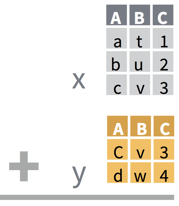
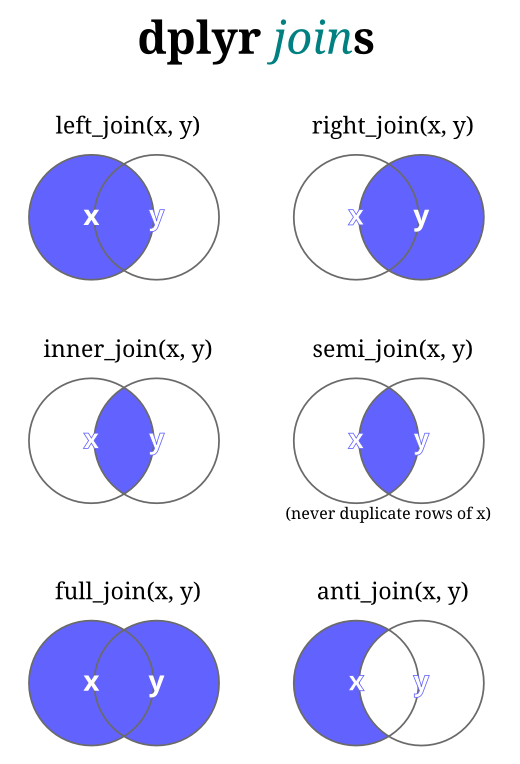
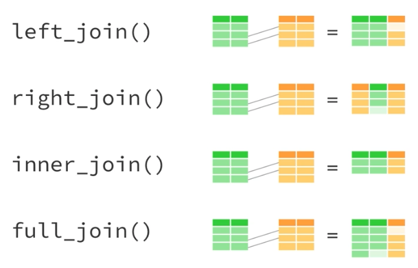
Joins: Our BERD workshop slides have another example that might visualize joins.
Slide 18 shows to datasets x and y, and what the resulting joins look like.
Slide 19 shows Venn diagrams of how the different joins behave.
pivot_longer makes plotting more understandable in an analysis sense, which situations would call for pivot_wider?
I tend to use pivot_longer() much more frequently. However, there are times when pivot_wider() comes in handy. For example, below is a long table of summary statistics created with group_by() and summarize(). I would use pivot_wider() to reshape this table so that I have columns comparing species or columns comparing islands.
The arguments of the pivot functions take some practice to get used to. I sometimes still pull up an example to remind me what I need to specify for the various arguments, such as the one mentioned above that I have used in workshops and classes.
We have not covered all the different arguments, and I recommend reviewing the help file and in particular the examples at the end of the page.
gt::gt()
The gt::gt package does make the tables look fancier, how do we add labels to those to have them look nice as well?
I highly recommend the gt webpage to learn more about all the different options to create pretty tables. Note the tabs at the top of the page for “Get started” and “Reference.”
See also section 3 of part 6 on “Side note about gt::gt()” for more on creating pretty tables.
here::here
would also love more examples of here() I am starting to understand it better but still am a little confused
I am still having trouble getting here() to work consistently. I was going to ask during class, but I think I am just not understanding how to manually nest my files correctly so that “here” works. I am struggling to get that set up correct, and thus, struggling to use it.
We’ll have some more examples in class, but I recommend reaching out to one of us (instructors or TA) to help you troubleshoot here::here.
Why we used full_join() in the class example instead of the other join options
In this case both datasets being joined had the same ID’s, and thus it did not matter whether we used left_join(), right_join(), full_join() or inner_join(). All of these would’ve given the same results.
Visualizing pivots and joins
pivot-longer is still hard for me to mentally visualize how it alters the dataset.
I always struggle to visualize pivots and joins.
Reshaping data take lots of practice to get the hang of, and something where I still pause while coding to think through how it will work and how to code it. Especially for pivoting, I often refer back to existing code I am familiar with. It’s normal at this point to still be muddy on these topics. Keep practicing though and read through some more examples.
 time  n   percent
  tp1 32 0.3333333
  tp2 32 0.3333333
  tp3 32 0.3333333
The goal was to create a factor variable of the character time point column called time with the levels 1 month, 6 months, and 12 months, instead of time’s values tp1, tp2, and tp3.
The code presented in class to accomplish this is below:
The question arose as to whether we could include factor() in the same step as case_when() when creating time_month above, instead of having to write it out as a second separate line in the mutate().
When using case_when(), we can do this as follows by piping the factor after the case_when():
What is new her is that we have not previously discussed labels.
You can think of the levels as the input for the factor() function.
It’s how we specify what the different levels are for the variable we are converting to factor, as well as the order we want the levels to be in.
If we do not specify the levels, then R will automatically use the different values of the variable being converted and arrange them in alphanumeric order. Example:
Note that both time_month4 and time_month5 started with the same levels.
Instead of using the labels option within factor() (the base R way), we can also accomplish this by using fct_recode() from the forcats package (loaded as a part of tidyverse):
# original tp levels:levels(mouse_data$time_month5)
%in% command, I feel like I understand but have some confusion and think it might just be one of those things I have to work with/apply to fully understand
We’ve used the %in% function in some examples, but I don’t think we’ve discussed it in detail.
The %in% function is used to test whether elements of one vector are contained in another vector. It returns a logical vector indicating whether each element of the first vector is found in the second vector.
Below are some examples that ChatGPT generated (and I slightly edited).
# Example 1: Using %in% with two numeric vectorsx <-c(1, 2, 3, 4, 5)y <-c(2, 4, 6)x %in% y
[1] FALSE TRUE FALSE TRUE FALSE
# Example 2: Using %in% with two character vectorsfruits <-c("apple", "banana", "orange", "grape")selected_fruits <-c("banana", "grape", "kiwi")selected_fruits %in% fruits
[1] TRUE TRUE FALSE
# Example 3: Using %in% with dataframe columnslibrary(tidyverse)# Create a dataframedf <-tibble(ID =c(1, 2, 3, 4, 5),fruit =c("apple", "banana", "orange", "grape", "kiwi"))df
# A tibble: 5 × 2
     ID fruit
  <dbl> <chr>
1     1 apple
2     2 banana
3     3 orange
4     4 grape
5     5 kiwi
# Filter rows where 'fruit' column contains values from selected_fruitsselected_fruits <-c("banana", "grape", "kiwi")df_filtered <- df %>%filter(fruit %in% selected_fruits)df_filtered
# A tibble: 3 × 2
     ID fruit
  <dbl> <chr>
1     2 banana
2     4 grape
3     5 kiwi
Clearest points
This class was all really clear. It was helpful to be reviewing some of the things we learned last week.
I appreciate the new codes on how to clean/reshape/combine messy data. I think that was the hardest parts to do in the other Biostatistics courses during projects.
Data cleaning
Most of the data cleaning exercises.
different strategies to clean data sets
The data cleaning made a lot of sense but I think I will struggle with solving problems in a really inefficient way.
Everything before Challenge 3
methods to merge datasets to create a table
inner join and full join are the same if all vectors are the same.
Pivot
ggplot and how to code data in to display what we want to display
Other comments
Is there a difference between summarize (with z) and summarise (with s)?
Great question!
In English, summarize is American English and summarise is British English. * In R they work the same way. The reference page for summarise() lists them as synonyms.
In R code I see summarise more, and now keep mixing up which is American and which is British.
In general, R accepts both American and British English, such as both color and colour.
Thank you for the survey reminders! The pace of the class feels much better compared to the pace at the beginning of the term
Thanks for the feedback!
I really enjoyed the walk through from start to finish of how to clean the data sheet and it really helped clear up many of the commands I was previously confused about
Thanks for the feedback! Glad the data wrangling walk through was helpful.
Week 8 (Part 7)
When loading a dataset, what does mean?
This occurs when you use the data() function to load a data set from a package. Per the help on this function (?data):
data() was originally intended to allow users to load datasets from packages for use in their examples, and as such it loaded the datasets into the workspace .GlobalEnv. This avoided having large datasets in memory when not in use: that need has been almost entirely superseded by lazy-loading of datasets.
data("iris") # this doesn't actually load the data set, but makes it available for usehead(iris) # Once it's used it will appear in the Environment as an object.
This was where we created a function to load 3 data sets, clean them, and convert them to long format. These are tasks we’ve seen in previous classes. In this challenge, the main takeaway was to see the DRY (Don’t repeat yourself) concept at play. Instead of writing the code 3 times for each data set, we can create a function where we only write the cleaning code once, then use that function 3 times.
Reviewing the challenge solutions and taking more time to work through it on your own is a good idea. We went through it pretty quick in class. You won’t usually be limited on time to get a function like that to work. In practice, if it’s taking more time and too complicated, then it’s fine to duplicate code so that you know it’s working correctly. But, with very repetitive tasks, functions can make your code less prone to errors from copying and pasting.
If you have trouble getting your code to work for the challenges, office hours are great for helping to debug code. Else, sharing full code in an email or on Slack.
purrr::pluck
There was a specific question:
purrr::pluck seems really useful, I wonder if you can tell it to pluck a specific record_ID?
The short answer is no. Not a specific ID. But if you know the position of the specific ID then you could.
# A tibble: 10 × 3
   id    sex     age
   <chr> <chr> <int>
 1 0001  M        22
 2 0002  M        32
 3 0003  F        64
 4 0004  F        32
 5 0005  M        23
 6 0006  M        49
 7 0007  F        49
 8 0008  M        29
 9 0009  M        26
10 0010  M        29
# Say we want to extract ID 0003.# With purrr::pluck we need to know that it's in the 3rd row of the ID columnpurrr::pluck(df, "id", 3)
[1] "0003"
# Gives an errorpurrr::pluck(df, "id", "0003")
NULL
# More than likely in this scenario, you would use a filter:df |> dplyr::filter(id =="0003")
# A tibble: 1 × 3
  id    sex     age
  <chr> <chr> <int>
1 0003  F        64
purrr::pluck was created to work with deeply nested data structures. Not necessarily data frames; there’s probably a more appropriate function out there for the task.
Lists – general confusion
What do we do with lists?
Using lists
We will get to work more with lists in Week 9 and get more opportunities to see how they are used.
Lists are more flexible and have the ability to handle various data structures which make them a powerful tool for organizing, manipulating, and representing complex data in R.
Lists – One bracket versus two brackets.
One bracket [ ] and two brackets [[ ]] serves different purposes, primarily when accessing elements in a data structure like vectors, lists, or data frames.
One Bracket [ ]:
Vectors:
When used with a single bracket, you can use it to subset or extract elements from a vector.
# Example with a vectormy_vector <-c(1, 2, 3, 4, 5)my_vector[3] # Extracts the element at index 3
[1] 3
Data Frames:
When used with a data frame, it can be used to extract columns or rows.
# Example with a data framedf <- tibble::tibble(name =c("Alice", "Bob", "Charlie"), age =c(25, 30, 22) )# Extract the age columndf["age"]
# A tibble: 3 × 1
    age
  <dbl>
1    25
2    30
3    22
Two Brackets [[ ]]:
Lists:
When working with lists, double brackets are used to extract elements from the list. The result is the actual element, not a list containing the element.
# Example with a listmy_list <-list(1, c(2, 3), "four")my_list[[2]] # Extracts the second element (a vector) from the list
[1] 2 3
Compare to using []
my_list[2]
[[1]]
[1] 2 3
[[]] returned the vector contained in that slot. [] returned a list containing the vector.
Nested Data Structures:
For accessing elements in nested data structures like lists within lists.
# Example with a nested listnested_list <-list(first =list(a =1, b =2), second =list(c =3, d =4))nested_list
nested_list[[1]] # Extract the list contained in the first slot
$a
[1] 1

$b
[1] 2
nested_list[[1]][["b"]] # Extracts the value associated with "b" in the first list
[1] 2
In summary, one bracket [ ] is used for general subsetting, whether it’s extracting elements from vectors, columns from data frames, or specific elements from lists. On the other hand, two brackets [[ ]] are specifically used for extracting elements from lists and accessing elements in nested structures.
How and when to use curly curly within a function
{{ }} will be covered in upcoming class lectures. We talked about it in Week 8 as a quick aside because a specific question came up. Not much detail was given intentionally as it is a separate topic for another day.
Week 9 (Part 7)
Matrices
Not entirely sure how to read or make sense of matrices yet (maybe I should have payed more attention in algebra), like when we saw the structure of a matrix here in the class script: str(output_model$coefficients)
In R, matrices are two-dimensional data structures that can store elements of the same data type. They are similar to vectors but have two dimensions (rows and columns). They are widely used in various statistical and mathematical operations, making them a fundamental data structure in the R.
Basic way to create matrices
# Create a matrix with values filled column-wise(mat1 <-matrix(1:6, nrow =2, ncol =3, byrow =FALSE))
     [,1] [,2] [,3]
[1,]    1    3    5
[2,]    2    4    6
# Create a matrix with values filled row-wise(mat2 <-matrix(1:6, nrow =2, ncol =3, byrow =TRUE))
# Accessing entire row or columnrow_vector <- mat1[1, ] # Entire first rowrow_vector
[1] 1 3 5
col_vector <- mat1[, 2] # Entire second columncol_vector
[1] 3 4
Convert to data.frame
as.data.frame(mat1)
  V1 V2 V3
1  1  3  5
2  2  4  6
library(tibble)tibble::as_tibble(mat1)
Warning: The `x` argument of `as_tibble.matrix()` must have unique column names if
`.name_repair` is omitted as of tibble 2.0.0.
ℹ Using compatibility `.name_repair`.
# You can also name the columns (and the rows)colnames(mat1) <-c("a", "b", "c")mat1
     a b c
[1,] 1 3 5
[2,] 2 4 6
tibble::as_tibble(mat1)
# A tibble: 2 × 3
      a     b     c
  <int> <int> <int>
1     1     3     5
2     2     4     6
for() loops
Still a little confused about the for() loops…
For loops are a staple in programming languages, not just R. They are used when we want to repeat the same operation (or a set of operations) several times.
The basis syntax in R looks like:
for (variable in sequence) {# Statements to be executed for each iteration}
Here’s a breakdown of the components:
variable: This is a loop variable that takes on each value in the specified sequence during each iteration of the loop.
sequence: This is the sequence of values over which the loop iterates. It can be a vector, list, or any other iterable object.
Loop Body: The statements enclosed within the curly braces {} constitute the body of the loop. These statements are executed for each iteration of the loop.
Using a copy and paste method to calculate the mean of each column would look something like this:
median(df$a)
[1] 0.579455
median(df$b)
[1] 0.07901281
median(df$c)
[1] -0.2194695
median(df$d)
[1] 0.3230435
But this breaks the rule of DRY (“Don’t repeat yourself”)
output <-c() # vector to store the results of the for loopfor (i inseq_along(df)) { output[i] <-median(df[[i]])}output
[1] 0.57945504 0.07901281 -0.21946947 0.32304348
For loops in R are commonly used when you know the number of iterations in advance or when you need to iterate over a specific sequence of values. While for loops are useful, R also provides other ways to perform iteration, such as using vectorized operations (example below) and functions from the apply family (not covered). It’s often recommended to explore these alternatives when working with R for better code efficiency and readability.
# With a for loopresult_addition_for_loop <-c()for (i in1:length(vector1)) { result_addition_for_loop[i] <- vector1[i] + vector2[i]}result_addition_for_loop
[1] 7 9 11 13 15
na.rm vs na.omit
Is there a difference between na.rm and na.omit?
Yes, there is a difference. In R, they are used in different context.
na.rm (Remove)
na.rm is an argument found in various functions (e.g. mean(), sum(), etc.) that allows you to specify whether missing values (NA or NaN) should be removed before performing the calculation.
From the help for mean() (?mean): a logical evaluating to TRUE or FALSE indicating whether NA values should be stripped before the computation proceeds.
# A vector with NA valuesvalues_with_na <-c(1, 2, 3, NA, 5)mean(values_with_na, na.rm =FALSE) # Result will be NA
[1] NA
# Excluding NA valuesmean(values_with_na, na.rm =TRUE) # Result will be (1+2+3+5)/4 = 2.75
[1] 2.75
na.omit (Omit missing)
na.omit is a function that can be used to remove rows with missing values (NA) from a data frame or matrix.
# Creating a data frame with NA valuesdf <-data.frame(A =c(1, 2, NA, 4), B =c(5, NA, 7, 8))# NAs in the columns of the data framedf
   A  B
1  1  5
2  2 NA
3 NA  7
4  4  8
# Using na.omit to remove rows with NA valuesdf |>na.omit()
  A B
1 1 5
4 4 8
purrr::map()
I am still a little foggy on the formatting of purrrmap and how to utilize it effectively.
The purrr::map function is used to apply a specified function to each element of a list or vector, returning the results in a new list.
Basic Syntax:
purrr::map(.x, .f, ...)
.x: The input list or vector.
.f: The function to apply to each element of .x.
...: Additional arguments passed to the function specified in .f.
Key Features:
Consistent Output:
map returns a list, ensuring a consistent output format regardless of the input structure.
Function Application:
The primary purpose is to apply a specified function to each element of the input .x.
Formula Interface:
Supports a formula interface (~) for concise function specifications.
purrr::map(.x, ~ function(.))
Example:
# Sample listmy_list <-list(a =1:3, b =c(4, 5, 6), c =rnorm(n =3))my_list
In this example, the map function applies the squaring function (~ .x ^ 2) to each element of the input list my_list. The resulting squared_list is a list where each element is the squared version of the corresponding element in my_list.
The purrr::map function is particularly useful when working with lists and helps to create cleaner and more readable code, especially in cases where you want to apply the same operation to each element of a collection.
General references
Is there a good dictionary type document with “R language” or very basic function descriptions? … find it difficult to know what functions I need because it is hard to recall their name or confuse it with a different function.
R Documentation (Built-in Help): R itself provides built-in documentation that you can access using the help() function or the ? operator. For example, to get help on the mean() function, you can type help(mean) or ?mean in the R console.
R Manuals and Guides: The official R documentation, including manuals and guides, is available on the R Project website: R Manuals.
R Packages Documentation: Many R packages come with detailed documentation. You can find documentation for a specific package by visiting the CRAN website (Comprehensive R Archive Network) and searching for the package of interest.
Online Resources: Websites like RDocumentation provide a searchable database of R functions along with their documentation. You can search for a specific function and find details on its usage and parameters.
When you use a function or learn to use it, make notes to yourself using Google Doc or OneNote or something similar.
Week 10 (Part 8)
Confusion on details of purrr::map()
purrr::map() applies a function to each element of a vector or list and returns a new list where each element is the result of applying that function to the corresponding element of the original vector or list.
map(.x, .f, ..., .progress =FALSE)
.x the vector or list that you operate on
.f the function you want to apply to each element of the input vector or list. This function can be a built-in R function, a user-defined function, or an anonymous function defined on the fly.
Simple example
library(tidyverse)# Example listnumbers <-list(1, 2, 3, 4, 5)numbers
# Using map to square each element of the listsquared_numbers <- purrr::map(.x = numbers, .f =~ .x ^2)
In this example: - numbers is a list containing numbers from 1 to 5. - ~ .x ^ 2 is an anonymous function that squares its input. - map() applies this anonymous function to each element of the numbers list, resulting in a new list where each element is the square of the corresponding element in the original list.
After executing this code, the squared_numbers variable will contain the squared values of the original list:
Suppose we have a list of data frames where each data frame represents the sales data for different products. We want to calculate the total sales for each product across all the data frames in the list.
# Sample list of data framessales_data <-list(product1 =data.frame(month =1:3, sales =c(100, 150, 200)),product2 =data.frame(month =1:3, sales =c(120, 180, 220)),product3 =data.frame(month =1:3, sales =c(90, 130, 170)))sales_data
Create a function `and apply it to each slot insales_data` list:
# Function to calculate total sales for each data framecalculate_total_sales <-function(df) { total_sales <-sum(df$sales)return(total_sales)}# Applying the function to each data frame in the listtotal_sales_per_product <- purrr::map(.x = sales_data, .f = calculate_total_sales)
In this example: - sales_data is a list containing three data frames, each representing the sales data for a different product. - calculate_total_sales() is a function that takes a data frame as input and calculates the total sales for that product. - map() applies the calculate_total_sales() function to each data frame in the sales_data list, resulting in a new list total_sales_per_product, where each element is the total sales for a specific product across all months.
After executing this code, the total_sales_per_product variable will contain the total sales for each product:
So, total_sales_per_product is a named list where each element represents the total sales for a specific product across all the data frames in the original list.
purrr::reduce()
How does it compare to purrr::map()?
The big difference between map() and reduce() has to do with what it returns:
map() usually returns a list or data structure with the same number as its input; The goal of reduce() is to take a list of items and return a single object.
# Using reduce to calculate cumulative sumcumulative_sum <- purrr::reduce(.x = numbers, .f =`+`)
In this example: - numbers is the vector we want to operate on. - The function + is used as the operation to perform at each step of reduction, which in this case is addition. - reduce() will start by adding the first two elements (1 and 2), then add the result to the third element (3), and so on, until all elements have been processed.
After executing this code, the cumulative_sum variable will contain the cumulative sum of the numbers:
We can combined the data sets in the list with reduce() and bind_rows()
# Using an anonymous function, note bind_rows takes 2 arguments.combined_sales_data <- purrr::reduce(.x = sales_data, .f =function(x, y) bind_rows(x, y))# Using a named functioncombined_sales_data <- purrr::reduce(.x = sales_data, .f = dplyr::bind_rows)
In this example: - We use an anonymous function within reduce() that takes two arguments x and y, representing the accumulated result and the next element in the list, respectively. - Inside the anonymous function, we use bind_rows() to combine the accumulated result x with the next element y, effectively stacking them on top of each other. - reduce() applies this anonymous function iteratively to the list of data frames, resulting in a single data frame combined_sales_data that contains the combined sales data for all products.
the list.files() function is used to obtain a character vector of file names in a specified directory. Here’s a breakdown of how it works and its common parameters:
Directory Path: The primary argument of list.files() is the path to the directory you want to list files from. If not specified, it defaults to the current working directory.
Pattern Matching: pattern is an optional argument that allows you to specify a pattern for file names. Only file names matching this pattern will be returned. This can be useful for filtering specific types of files.
Recursive Listing: If recursive = TRUE, the function will list files recursively, i.e., it will include files from subdirectories as well. By default, recursive is set to FALSE.
File Type: The full.names argument controls whether the returned file names should include the full path (if TRUE) or just the file names (if FALSE, the default).
Character Encoding: You can specify the encoding argument to handle file names with non-ASCII characters. This argument is especially useful on Windows systems where file names may use a different character encoding.
Here’s a simple example demonstrating the basic usage of list.files():
# List files in the current directoryfiles <-list.files()# Print the file namesprint(files)
This will print the names of all files in the current working directory.
#| eval: false# List CSV files in a specific directorycsv_files <-list.files(path ="path/to/directory", pattern ="\\.csv$")# Print the CSV file namesprint(csv_files)
character(0)
This will print the names of all CSV files in the specified directory.
Overall, list.files() is a handy function for obtaining file names within a directory, providing flexibility through various parameters for customization according to specific needs, such as filtering by pattern or handling file names with non-standard characters.
NOTE You need to pay attention to your working directory and your relative file paths. See Week 2 or 3 (?) about here package and the discussion about files paths. Best to always use Rprojects and the here package.
2023
Week 1
Pacing
Mean 3.18, IQR [3,3] so, that’s a good sign, though there was one comment it went a little fast. I admittedly was trying to cram in a lot of basics all at once, so I’ll try to go a touch slower with the hard things.
Muddiest Points
Remember, all of this is anonymous. I don’t post everything everyone says on here, but I do read them all and think about how to improve the class based on what everyone says.
Boolean data, until you explained it
We will talk more about boolean data in class 2, I kind of rushed the intro to that but we’ll definitely see more examples!
default arguments
I added this one, I want to make sure to show you the help in R and how we know what the “default” arguments are, that we don’t need to specify.
removing missing values
Yes this is a confusing thing in R, one point to remember is the difference between a function like na.omit() and an argument like na.rm = TRUE which sets the missing data behavior within a specific function like mean().
myvec <-c(1, NA, 3)# removes missing values, does not save your work!na.omit(myvec)
# removes missing values, overwrites the object/variable myvec after removing themmyvec <-na.omit(myvec)myvec <-c(1, NA, 3)# default behavior is to include NA in the computationmean(myvec)
[1] NA
# specifies that we want to get rid of NA firstmean(myvec, na.rm =TRUE)
[1] 2
# different functions have different arguments to handle missing data# see ?cor for help and the explanation of the use argumentvec1 <-c(1, NA, 2, 3)vec2 <-c(2, 3, NA, 4)cor(vec1, vec2)
[1] NA
cor(vec1, vec2, use ="pairwise.complete.obs")
[1] 1
# cor(vec1, vec2, use = "all.obs") # this throws an error, why?
Data types and vectors. It was clear, however, when I watched the class recording.
We will go over this again in class 2 when we talk about data!
While I was reading the materials about vectors and variables, I’m still not very clear on the differences between vectors and variables. For instance, when we concatenate a list of regions (example from book) and create a vector named “region.” It sounds similar to how we assign values or characters to create a variable
This is a great point, and I tend to be a little lax with the definitions of some of these terms so apologies if it is confusing.
I would say a variable is the same as an object in R. It is the name of something that we save and that we can see in our environment tab. That means it could be a vector, a data set, a list, a unique object type – all data types we will talk about in the coming classes.
I also use the word “variable” when talking about columns of a data set or data frame, though. Therefore, it’s not a precise word and I’m sorry I use it so much!
A vector is a specific type of object in R. It has a length and a class/type. It does not have a “width” like a data frame does (we will talk about these in class 2). We will also talk about types or classes of vectors (character, numeric, boolean) a bit more in these classes.
For a more thorough introduction, read R for Data Science Vector. If you want a rather advanced treatment of data types, see Advanced R.
As far as naming vectors or data, we often call them something that we can easily remember or make sense of. I think that also can cause confusion though, in the regions example.
This all make more sense once we talk about data frames, which contain vectors as columns!
packages - why did my R crash?
Ugh I’m so sorry and I don’t have a clear idea. My best guess is that there were older packages installed and for some reason pacman::p_load tried to install packages without installing their dependencies first packages that the installed package relies on to work, and often need at least a certain version. Perhaps if you don’t update your packages all that often, install.packages() is the safer option?
The options for code blocks in r markdown
I didn’t talk about this much yet, but I will keep showing examples of this. In the meantime, here are some good references, that I often have to go back to because I forget most of them most of the time:
I will also try to mention global options in class 2 as well.
how to also have an output below my code chuck as well
I’ll talk about this again/more as well. This is a YAML option, and can be set using the “gear” icon next to the “Knit” button at the top of an Rmd (Chunk Output Inline vs Chunk Output Console). I think we can’t have it both ways. Also note that table output will look different from interactive R markdown and knitted R markdown sometimes. That can be a point of confusion. You can also change how that looks in “Output Options” from that gear dropdown menu (General -> print data frames as:)
R markdown in general, also R studio projects
Understandable, I threw a lot of new stuff at most of you, and I’ll focus more on these things in class 2! I haven’t shown you the full benefits of using Rstudio projects yet because we haven’t started working with data. But hopefully class 2 and 3 it will become a bit more clear.
Clearest Points
Lots of things here I’m not including, but, thank you for all of it!
Concatenate! I have never known what c() stood for!
It’s a weird one, for sure!
First time real exposure to R, so I REALLY was amazed by knitting the Rmd and how the class content was all “interactively” set in the Rmd.
It’s one of the main reasons why I just start using Rmd right away, because it’s pretty neat. It might cause more headaches later because it takes time getting used to, but it’s worth it to me.
Other messages, just a selection
Lots of you liked having challenges. Sometimes I get carried away adding too much instruction because there is so much I want to show you, so I hope I provide enough time for challenges this year.
i’ve had R experience but it’s difficult for me to quickly learn and adapt to it. I understand how to use it but have difficulty creating things like tables or organizing data. I’m hoping by the end of this course, i’ll be able to gain more knowledge to allow me to do those types of task.
You are my perfect audience, these are my goals, too!
After 2 years of just sort of flinging myself at R willy-nilly, the first class showed me a lot of tips for using R that have already made my life easier.
So happy to hear it!
Week 2
Muddiest Points
the benefits of tibble vs data frame and when to use which?
In this class we will always use tibble. Just remember that an object can be multiple types. A tibble is a data frame, but not vice versa. A tibble is really a data frame with “perks”. See this explanation from the tibble 1.0 package release
There are two main differences in the usage of a data frame vs a tibble: printing, and subsetting.
Tibbles have a refined print method that shows only the first 10 rows, and all the columns that fit on screen. This makes it much easier to work with large data. In addition to its name, each column reports its type, a nice feature borrowed from str():
Another interesting difference is that tibbles don’t have row names, but a lot of built in data.frames in R do. But rownames are hard to get out. So, when you make a tibble of a data.frame you can tell the function to use the rownames as a column:
Tibbles also clearly delineate [ and [[: [ always returns another tibble, [[ always returns a vector. No more drop = FALSE!
If we ask for the first column using the [] notation, we receive a numeric vector from a data frame, and a tibble/data.frame from the tibble.
We have not learned the [[]] yet because we have not talked about lists in R, but we will soon. The code below returns the first column as a vector for both a data frame and a tibble.
As I was mentioning in class, there are some (older) functions that don’t like tibbles, but all you need to do is just make its primary class a data.frame as such:
A handful of functions are don’t work with tibbles because they expect df[, 1] to return a vector, not a data frame. If you encounter one of these functions, use as.data.frame() to turn a tibble back to a data frame:
path files and knowing if you’re in a project or just an RMD
R markdown vs R projects
I hope to spend more time talking about this in class 4.
ggplot stuff was the most muddy, but I also haven’t done a lot of ggplot stuff before
Yes this was definitely expected for a brief intro, ggplot takes a while to get the hang of! We will use ggplot every class now, so we will go through it in bite sized pieces.
Using na=“NA” to pull in data and how to know that it’s needed.
I will show more examples of this. Rule number one of importing data in any software is to look at your data, and figure out if what you see in the software is what you expect. Always look at your data! The read_excel(filename, na="NA") is a strange case that isn’t actually very common to code data as “NA” directly, but I wanted to show you how it looks different when it does happen. Usually, missing data is just a blank space, which is automatically read in as the special NA data type in R.
# If you did not include `na=NA` it would have been read in like thisdf1 <-tibble(a =c("NA","C","D"), b=1:3, c =c(1,3,"NA"))# If you did include `na = NA` it would have been read in like thisdf2 <-tibble(a =c(NA,"C","D"), b=1:3, c =c(1,3,NA))# note the character types of the two DFs, and the way NA is printeddf1
# A tibble: 3 × 3
  a         b c
  <chr> <int> <chr>
1 NA        1 1
2 C         2 3
3 D         3 NA
df2
# A tibble: 3 × 3
  a         b     c
  <chr> <int> <dbl>
1 <NA>      1     1
2 C         2     3
3 D         3    NA
I saw a lot of code with the two colons (“::”) in the middle. It is unclear to me if this is an alternative way to write some commands or if there is a certain context in which it is used.
Good question, what this does is pulls a function from a package, so it works whether you have loaded the package (using library() or p_load()) or not. I mainly use it as a clue to you to where the function is coming from. Otherwise, you may not know you need to load that package to use it! For instance:
# does not work, haven't loaded the package janitormtcars %>%tabyl(am, cyl)
# does workmtcars %>% janitor::tabyl(am, cyl)
 am 4 6  8
  0 3 4 12
  1 8 3  2
# also workslibrary(janitor)mtcars %>%tabyl(am, cyl)
 am 4 6  8
  0 3 4 12
  1 8 3  2
Clearest Points
skim
loading our excel to R studio
Loading in the data and selecting the sheets that are most relevant to what we are looking to do was very clear and a nice foundation for future projects. I found that showing different ways of importing the data was helpful.
I’m glad, the import tool in Rstudio is very nice, just remember to save the code in your Rmd.
functionality of ggplot
tidying the data
Found out what eval=TRUE and eval=FALSE mean!
Great and I’ll show that again for anyone who was confused! (“still a little bit confused about the {r, EVAL} code”)
Other messages
Some people had trouble getting the fig.path= to work in the knitr options. I’m not sure what could be causing that but feel free to ask me during break.
link to the course website that is in the overview tab in SAKAI links to last years materials.
Oops thank you great catch, fixed!
Speed is going great. I’m just worried as we progress through the course, it’ll be more difficult. Overall, really enjoying this class.
I understand the concern, some things will get more difficult (I’m thinking across() in class 4, writing functions, and purrr), but we will also circle back to some things that might be familiar or maybe less complicated to start (stats models, making tables). Definitely keep asking questions and I will slow down as needed!
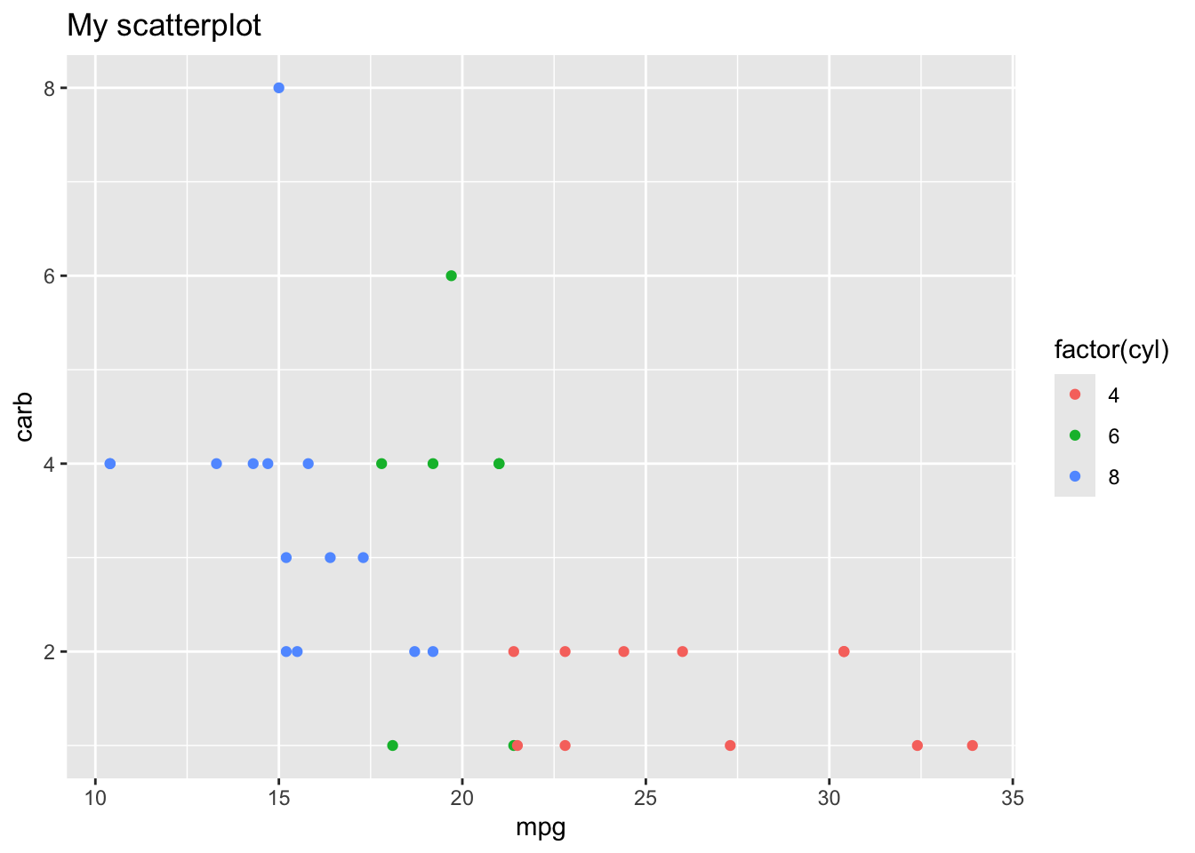
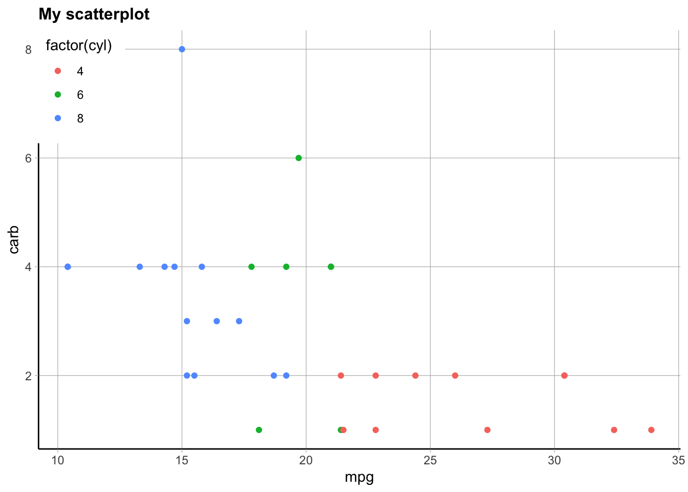
Here’s a couple examples using this one plot, so you can see how the theme changes the look of the figure, when you use built in themes from the ggplot2 package (yes it only works in ggplot figures, for the person who asked about that)
library(tidyverse)p <-ggplot(mtcars, aes(x = mpg, y = carb, color =factor(cyl))) +geom_point() +labs(title ="My scatterplot")p
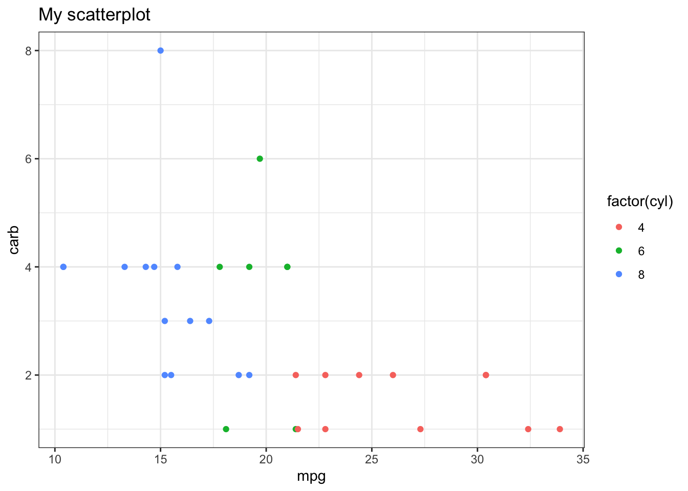
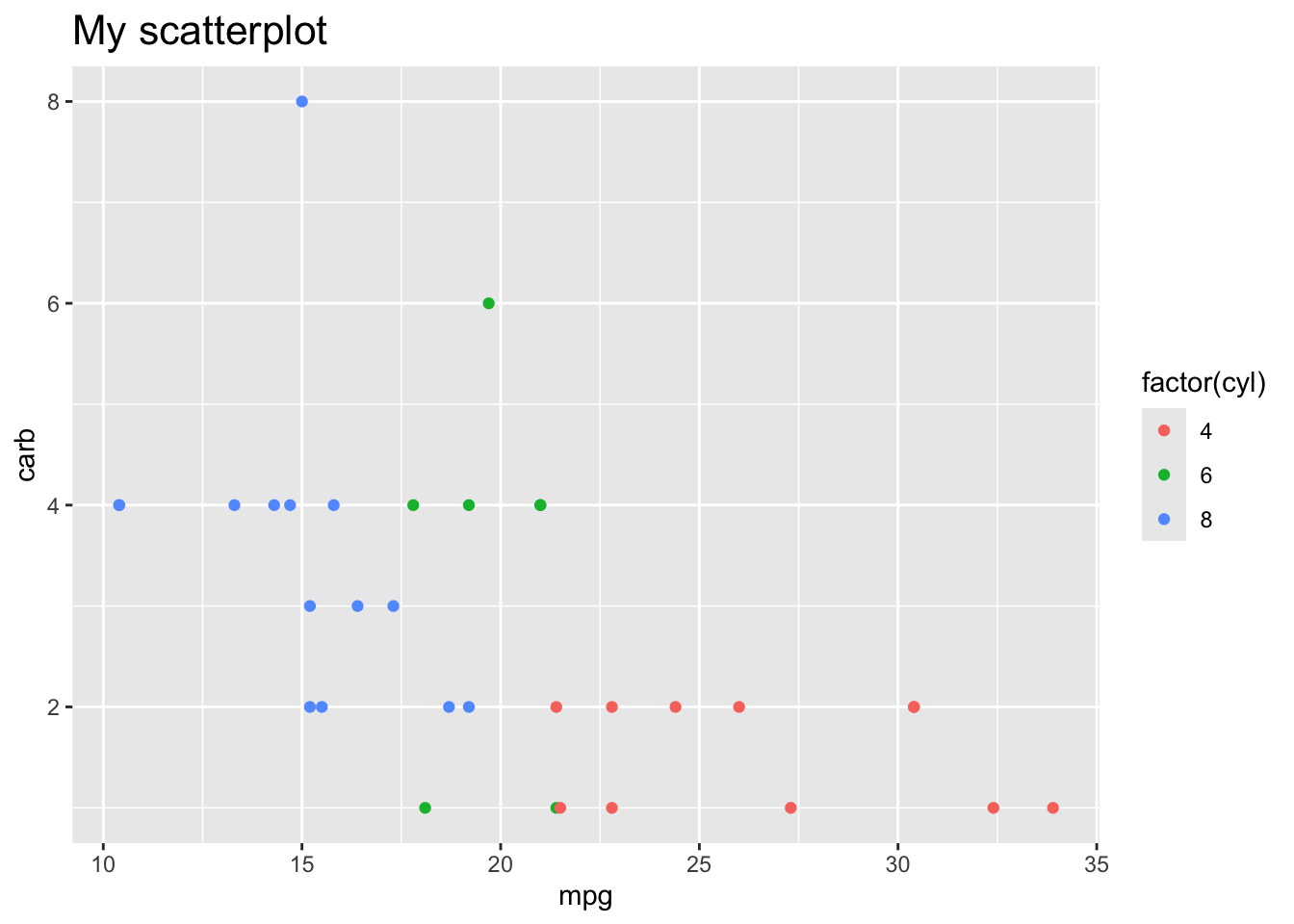
Here are some built in themes:
p +theme_bw()
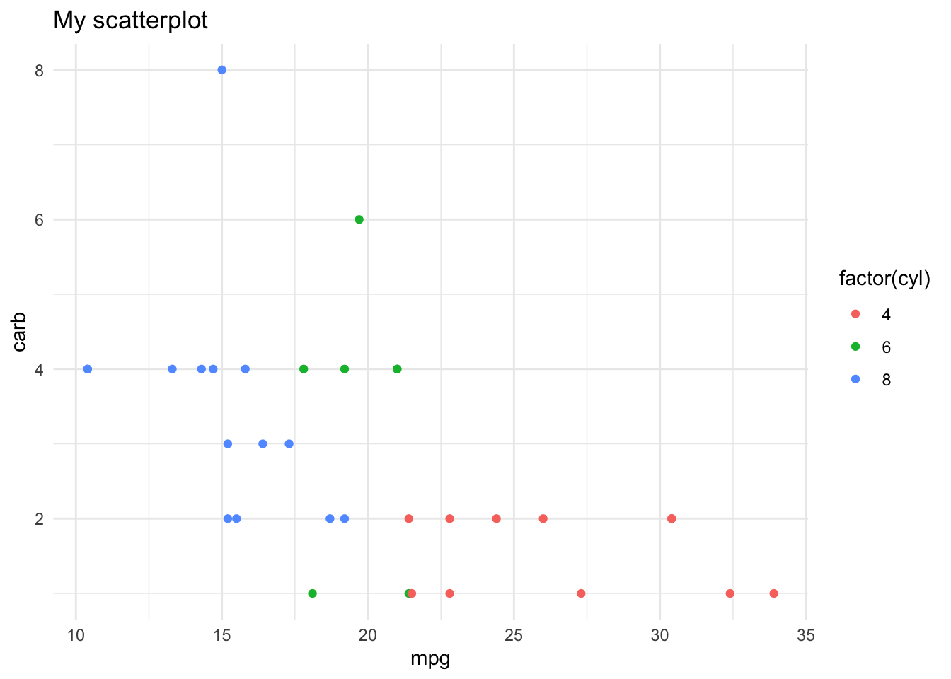
p +theme_minimal()
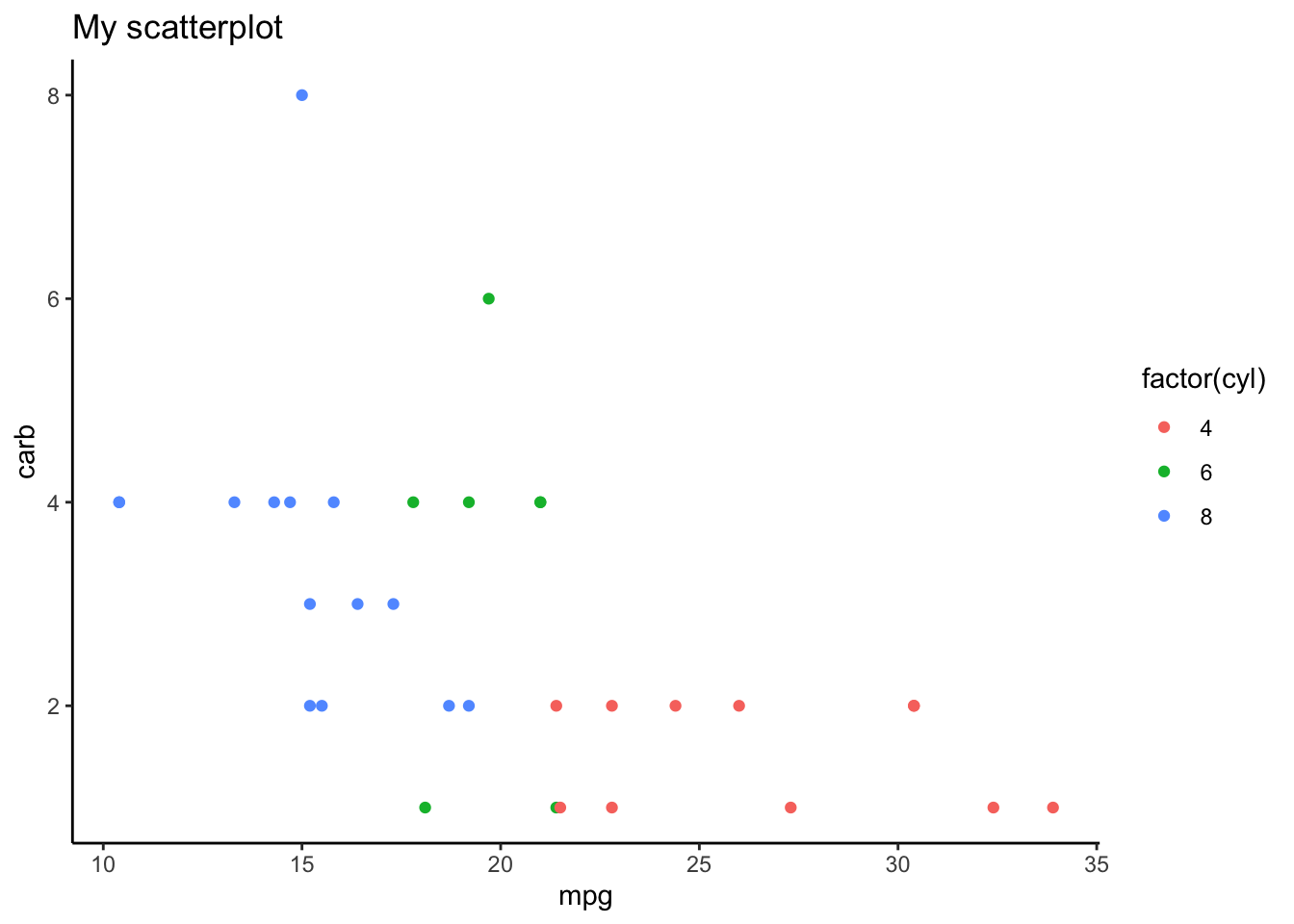
p +theme_classic()
However you can make more customized themes or plot changes where you use the theme() function to add in a lot of other elements. You can use this add on function to choose specific parts of the plot that you want to change, like this example from the above reference. Anything specified here will override the built in theme selected first. There are many options, and looking at specific examples will help. I am always, always googling how to change parts of the theme/plot like this, because there are just so many options it’s too hard to remember them all.
Warning: The `size` argument of `element_line()` is deprecated as of ggplot2 3.4.0.
ℹ Please use the `linewidth` argument instead.
Warning: The `size` argument of `element_rect()` is deprecated as of ggplot2 3.4.0.
ℹ Please use the `linewidth` argument instead.
Warning: A numeric `legend.position` argument in `theme()` was deprecated in ggplot2
3.5.0.
ℹ Please use the `legend.position.inside` argument of `theme()` instead.
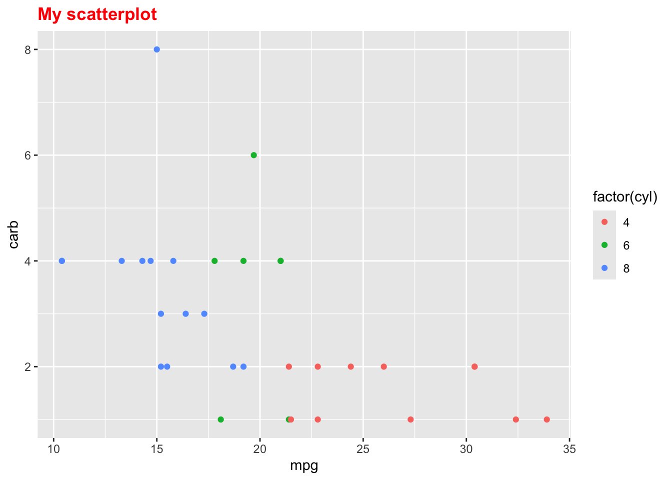
Here’s a simpler example just changing the title (from the above reference):
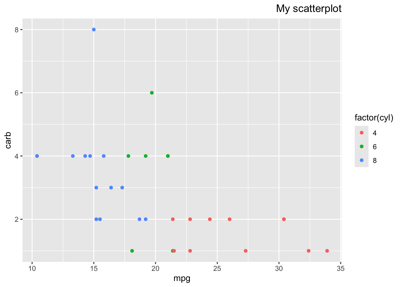
p +theme(plot.title =element_text(size =16))
p +theme(plot.title =element_text(face ="bold", colour ="red"))
p +theme(plot.title =element_text(hjust =1))
here()
Agreed, it’s very confusing, more in class 4!
Could you please clarify about the use of select(one_of) and the count command that was mentioned in dplyr cheatsheet?
These are very different, if you are talking about select() vs count(). One thing to note is that since I recorded that class, one_of() has been superseded/replaced by any_of() and all_of().
First, select() is a function to subset columns.
library(palmerpenguins)
Here we specify the columns we want in the order we want:
penguins %>%select(bill_length_mm, island, species, year)
Warning: Using an external vector in selections was deprecated in tidyselect 1.1.0.
ℹ Please use `all_of()` or `any_of()` instead.
  # Was:
  data %>% select(colnames_needed)

  # Now:
  data %>% select(all_of(colnames_needed))

See <https://tidyselect.r-lib.org/reference/faq-external-vector.html>.
But the key about any_of and all_of is what it allows. any_of() allows column names that don’t exist! Using no tidyselect helper or all_of() does not allow this. Which you use depends on what you want to allow to happen.
colnames_needed <-c("bill_length_mm","island","species","year","MISSING")# penguins %>% select((colnames_needed)) # does not workpenguins %>%select(any_of(colnames_needed)) # works!
On the other hand, count() is mainly to count the number of unique values in a column/vector:
penguins %>%count(species)
# A tibble: 3 × 2
  species       n
  <fct>     <int>
1 Adelie      152
2 Chinstrap    68
3 Gentoo      124
This created a new tibble, that summarizes the species column by counting the number of each type of species. This works for any type of vector but is most useful with character and factor columns. You can also use multiple columns here to see all possible combinations:
Super! I want to take the time to mention (and hopefully not confuse everyone) that the pipe has recently (2021) been integrated into “base R”, that is, it’s loaded without loading the tidyverse package. HOWEVER it is this symbol |> and does not behave exactly like the tidyverse pipe %>% (actually from the magrittr package within the tidyverse package). For all the usual uses it works the same, so it could be used interchangeably in this class. Just know that if you see that type of pipe being used, assume it’s doing basically the same thing. Even R for Data Science is likely moving to use the native/base pipe, see this explanation. Probably next year’s class I will switch everything over to use this, though I still just use %>% in my own work as it’s slightly more flexible for more “advanced” usage.
I’ve noticed some confusion about what I call “saving your work”, so we’ll go over these slides.
using factors, what you’re doing and the benefit of turning things into factors in mutate
I usually turn something into a factor for plotting (especially if I have a categorial numeric variable), and we’ll see more examples of that. We also later will see how it matters in statistical modeling/regression. It also is often easier to manage levels/categories this way, as we will see when we talk about the forcats package again in class 6.
case_when is not easy
Correct! Also some other comments on wanting more practice with case_when(). We will continue to see examples with this as we finish part5 and in other classes. It’s a very handy function so I use it a lot! See also the video above about factors with another explanation.
The function for converting a vector back from factor to character - I thought I had it, but I didn’t.
Oh, I didn’t show this!
# make a character vectormyvec <-c("medium", "low", "high", "low")myvec_fac <-factor(myvec)myvec_fac
[1] medium low    high   low
Levels: high low medium
class(myvec_fac)
[1] "factor"
# get the levels outlevels(myvec_fac)
[1] "high" "low" "medium"
# Note we can "test" the classes of something like so:is.factor(myvec_fac)
[1] TRUE
is.character(myvec_fac)
[1] FALSE
# Now we can change it backmyvec2 <-as.character(myvec_fac)myvec2
[1] "medium" "low" "high" "low"
class(myvec2)
[1] "character"
levels(myvec2) # no levels, because it's not a factor
NULL
# we could also change to numeric, how do you think it picks which number is which?myvec3 <-as.numeric(myvec_fac)myvec3
[1] 3 2 1 2
# levels in order is assigned 1, 2, 3table(myvec_fac, myvec3)
myvec3
myvec_fac 1 2 3
high 1 0 0
low 0 2 0
medium 0 0 1
# change the level ordermyvec_fac2 <-factor(myvec, levels =c("low", "medium", "high"))levels(myvec_fac2)
[1] "low" "medium" "high"
myvec4 <-as.numeric(myvec_fac2)myvec4
[1] 2 1 3 1
table(myvec_fac2, myvec4)
myvec4
myvec_fac2 1 2 3
low 2 0 0
medium 0 1 0
high 0 0 1
factor vs as.factor
Essentially the same. From the help documentation ?factor: “as.factor coerces its argument to a factor. It is an abbreviated (sometimes faster) form of factor.”
I would like to know when you recommend that we save a new data set once we create new covariates. Also, it is unclear to me how you add the variable to the existing data.
If I want to use that column/covariate again, I save it (so almost always, as I don’t often make a column without using it later). I usually save it back into the original data set I’m working with, that is, overwrite that object to be updated with the new column. As long as I keep track of my changes this is definitely ok. It can get confusing having too many versions of a data set floating around. If something is broken, the worst that happens is that you’ll just need to start from the beginning and reload your data (the data file will remain untouched) and re-run the code.
library(tidyverse)library(palmerpenguins)# does not save the new column, just prints resultpenguins %>%mutate(newvec = bill_length_mm/bill_depth_mm)
# saves new column in a data frame in the original data frame penguins# *overwrites penguins*penguins <- penguins %>%mutate(newvec = bill_length_mm/bill_depth_mm)glimpse(penguins)
We will talk more about palettes when we finish part4 but there are many, many. I suggest finding a package or two that has the palettes you like and working with those. See a bunch listed here (scroll down in the readme).. My favorites are ggthemes and colorBlindness.
I’m curious what the best practice is for stringing things together versus breaking them into pieces. For example, if I was trying to make a binary variable where all values were classified as larger or greater than the mean, I could use mean() inside several other functions like mutate(). Alternately I could calculate mean() [meanxx <- mean(xxx)] and save it as an object, and then use the other functions on that value. I’m curious because it seems like if you did too many functions at once and were getting errors, it would be hard to tell what was wrong. But if you did it in a more stepwise fashion, you could see (for example) that mean() wasn’t working because there were NAs in your dataset. More importantly, I think if you were getting an erroneous answer (not an error, but a wrong answer, like if you calculated the mean of a variable but your NA’s were marked with “-88” and so R considered these actual observations) you might not know if you joined too many functions together and didn’t “see” what was happening under the hood. I’m curious how to deal with that.
I copied over this whole question because I think it is an excellent one, and well said (hope you don’t mind)! I think this is something that evolves as you become more experienced in coding and debugging, and as you find your own style of coding. I will talk some about debugging later, but what you are saying about breaking things up into pieces absolutely helps with that.
The one thing to make sure of is that if you are saving intermediate steps, such as meanxx <- mean(mydata$xx) and using it later, but then you update the data set (filter, replace NAs, fix an incorrect data entry, whatever), you need to make sure to update/re-calculate that mean object as it no longer matches your newer data set! So there is more to keep track of, in that case.
I will say that if you are keeping track of all the steps well, then functionally it does not matter too much, so if it makes things easier to break it up, do that! If you like to chain everything together (often I do) you can run each piece by highlighting the code and running just that part to see what is going on, and this is something I do often.
Your example is something I would probably do, though, as using the mean inside mutate does make me a bit nervous. For example, let’s use median because it’s easier to check my work at the end:
library(janitor) # for tabyl()# there are NAs in here:median(penguins$body_mass_g)
[1] NA
# let's save the median as a vector of length 1, remove NAstmpmedian <-median(penguins$body_mass_g, na.rm =TRUE)tmpmedian
[1] 4050
penguins <- penguins %>%mutate(large_mass =case_when( body_mass_g >= tmpmedian ~"yes", body_mass_g < tmpmedian ~"no"# this allows NAs to remain NA ))penguins %>%tabyl(large_mass)
large_mass n percent valid_percent
no 170 0.494186047 0.497076
yes 172 0.500000000 0.502924
<NA> 2 0.005813953 NA
# if I had just used median without checking for NAs, they all are NA:penguins %>%mutate(large_mass =1*(body_mass_g >=median(body_mass_g))) %>%tabyl(large_mass)
large_mass n percent valid_percent
NA 344 1 NA
# Note if I just want females, this no longer makes sense:penguins %>%filter(sex=="female") %>%mutate(large_mass =case_when( body_mass_g >= tmpmedian ~"yes", body_mass_g < tmpmedian ~"no"# this allows NAs to remain NA )) %>%tabyl(large_mass)
large_mass n percent
no 107 0.6484848
yes 58 0.3515152
# but this would:penguins %>%filter(sex=="female") %>%mutate(large_mass =case_when( body_mass_g >=median(body_mass_g, na.rm =TRUE) ~"yes", body_mass_g <median(body_mass_g, na.rm =TRUE) ~"no" )) %>%tabyl(large_mass)
large_mass n percent
no 80 0.4848485
yes 85 0.5151515
Week 5
Muddiest points
I wasn’t super unclear about it, but just want to be more comfortable using summarize() and across and group_by functions. It looks like these will be really useful for future data projects, so that’s exciting! across function was a bit hazy because screen kept freezing
Sorry the zoom malfunctioned during this rather important and confusing section!
We will have more practice with across in other sections but the main points I want to get across (ha) are:
group_by() is used to “group the data” (a.k.a “split”) by a categorical variable, and then all kinds of computations can be done within groups including summarize() but also slice() (such as slice_sample()) and later we will see this with nest() etc.
summarize() can be used with or without group_by() to collapse a big data set into a summarized table/data frame/tibble. This is still data, it’s just summarized data. Be careful when you are saving it, don’t overwrite your original data.
across() can be used inside mutate() and summarize() to “select” the columns we want to transform/mutate or summarize
across() uses what we call “tidyselect” syntax. For explanation and examples you can type ?dplyr_tidy_select or go to this website.
the syntax of .x ~
We use this when we are creating our own function inside of mutate. Think of algebra, where if we want to add something we might say:
y = x + 3
y = x/10
y = log(x)
y = exp(x)^3 - x/10
This is the same idea, except it’s just written with the special syntax/variable name that R knows how to interpret, where we use .x instead of x:
y = .x + 3
y = .x/10
y = log(.x)
y = exp(.x)^3 - .x/10
But we also need to use ~ to tell R, here’s a function! and we use the argument name and equal sign .fns = to say, here we are inputting the custom function as the argument input. If you look at the help ?across we see this is called “A purrr-style lambda” because we use it in the purrr package functions as well (we will see this later):
# think of this as input to the argument of across()# typical argument syntax arg = _____.fns =~ .x+3.fns =~ .x/10.fns =~log(.x).fns =~exp(.x)^3- .x/10
And this needs to go inside the nested functions mutate(across()) as an argument: mutate(across(.cols = ----, .fns = ----)):
We can also apply multiple functions by putting them inside a list() and we can give them names:
# here we have 3 functionspenguins %>%mutate(across(.cols =c(bill_length_mm, body_mass_g),.fns =list(~ .x/3, log, # just using the named function, don't need .x~exp(.x)^3- .x/10))) %>%glimpse()
# here we have the same 3 functions but with namespenguins %>%mutate(across(.cols =c(bill_length_mm, body_mass_g),.fns =list(fn1 =~ .x/3,log = log,fn2 =~exp(.x)^3- .x/10))) %>%glimpse()
how do we change the names when using across() inside mutate()
I skipped this for the sake of time and to avoid confusion last class and showed you how to do this using rename() instead, but let’s go over it now a little bit.
The .names argument inside across() uses a function called glue() inside the package glue. We haven’t covered glue package syntax yet (it’s in part9) but think of it as a string concatenating (“gluing”) method where we write out what we want to be in the text string inside quotes, but use variable names and code functions inside of the quotes in a special way. The important part to know right now is that the stuff inside {} is code, and everything else is just text. Here when we use .col inside the glue code that is the stand-in for the column name, so "{.col}" is literally just the column name, and "{.col}_fun" is the column name with “_fun” appended to it.
Look at ?across and the .names argument for some info and the defaults.
# Does not change names of transformed columns# no longer accruate since not mmpenguins %>%mutate(across(.cols =ends_with("mm"), .fns =~ .x/10)) %>%glimpse()
# adds cm to end of column names, but still has mm, confusingpenguins %>%mutate(across(.cols =ends_with("mm"),.fns =~ .x/10,.names ="{.col}_cm")) %>%glimpse()
# code inside the {} is evaluated, # so we can use stringr::str_remove() to remove what we don't want there# str_remove_all() also works# note now we have kept the original columns as well# note we need single quotes for the glue code because we are wrapping it in# double quotes alreadypenguins %>%mutate(across(.cols =ends_with("mm"),.fns =~ .x/10,.names ="{str_remove(.col,'_mm')}_cm")) %>%glimpse()
# alternative that works here is using str_replace()penguins %>%mutate(across(.cols =ends_with("mm"),.fns =~ .x/10,.names ="{str_replace(.col,'_mm', '_cm')}")) %>%glimpse()
It’s unclear to me if there is distinction between using ‘str_remove_all’ and ‘separate()’ when we talked about removing “years old” from the column “age”. Are there particular circumstances where one is preferred over the other?
In R and in programming in general, there are always multiple ways to do the same thing. Often many, many ways! There is no preferred way just which makes the most sense to you/which you are most comfortable with.
For me, I like to use the stringr functions to remove stuff from columns that I don’t want, because it is the most “clear” to me and also probably to anyone reading my code.
The separate() way is more of a clever trick, an “out of the box” way to use an existing function that works for our needs in this case. There are a lot of things like that, and it’s perfectly ok to use them if you understand what they are doing and why.
arrange with two variables
Here’s a simple example so we can see how arrange() works with two categories (this is analogous to sorting by two variables in excel)
# A tibble: 4 × 4
id animal weight age
<int> <chr> <dbl> <dbl>
1 1 cat 10 15
2 2 mouse 1 3
3 3 dog 20 3
4 4 cat 8 20
mydata %>%arrange(weight)
# A tibble: 4 × 4
id animal weight age
<int> <chr> <dbl> <dbl>
1 2 mouse 1 3
2 4 cat 8 20
3 1 cat 10 15
4 3 dog 20 3
mydata %>%arrange(animal)
# A tibble: 4 × 4
id animal weight age
<int> <chr> <dbl> <dbl>
1 1 cat 10 15
2 4 cat 8 20
3 3 dog 20 3
4 2 mouse 1 3
# arrange by animal first, then weight within animal categoriesmydata %>%arrange(animal, weight)
# A tibble: 4 × 4
id animal weight age
<int> <chr> <dbl> <dbl>
1 4 cat 8 20
2 1 cat 10 15
3 3 dog 20 3
4 2 mouse 1 3
# does not do anything in this case, but would arrange by age if there were ties in the weight column within the animal categorymydata %>%arrange(animal, weight, age)
# A tibble: 4 × 4
id animal weight age
<int> <chr> <dbl> <dbl>
1 4 cat 8 20
2 1 cat 10 15
3 3 dog 20 3
4 2 mouse 1 3
stringr::str_to_title()
Just a clarification:
Remember to read help documentation and look at examples if still not clear!
str_to_title("hello")
[1] "Hello"
str_to_title("hello my name is jessica")
[1] "Hello My Name Is Jessica"
str_to_title("HELLO MY name is jessica")
[1] "Hello My Name Is Jessica"
There are other similar “case conversion” functions as well:
str_to_upper("HELLO MY name is jessica")
[1] "HELLO MY NAME IS JESSICA"
str_to_lower("HELLO MY name is jessica")
[1] "hello my name is jessica"
str_to_sentence("HELLO MY name is jessica")
[1] "Hello my name is jessica"
stringing together multiple commands in a pipe, which comes first and which functions are safe to put inside other functions- and if so- how do you know what order to put them in.
You’ll want to put them in the order that you want the operations to be performed.
For instance, if you want to summarize a data set after filtering, then put filter() first then summarize(). When in doubt, don’t string them together just do them one at a time!
Regarding which functions are safe to put inside other functions I am not sure exactly what you mean, but perhaps it’s the summarize(across()) type situation that is causing confusion. In this case, the result of across() becomes an argument input for summarize(). We also use functions as arguments inside across().
This part will require just more experience seeing what functions go where and getting used to all the syntax. I’ll try to point out specific examples where it makes sense to put functions inside other functions, but in general the tidyverse “verbs” such as mutate(), select(), filter(), summarize(), separate(), rename() are done in some kind of order that makes sense for how you want to transform your data, and they are chained together by pipes or done one at a time.
# mutate firstpenguins <- penguins %>%mutate(bill_length_cm = bill_length_mm/10)# create a filtered data sest of just female penguinspenguins_f <- penguins %>%filter(sex=="female")# we could have mutated *after* filtering in this case, it doesn't matter if we only care about the female penguins# summarize that female penguin data set, don't save as anything# just print it outpenguins_f %>%summarize(across( # across goes inside summarize.cols =where(is.numeric), # where() is a function inside across().fns = mean, na.rm =TRUE))
Warning: There was 1 warning in `summarize()`.
ℹ In argument: `across(.cols = where(is.numeric), .fns = mean, na.rm = TRUE)`.
Caused by warning:
! The `...` argument of `across()` is deprecated as of dplyr 1.1.0.
Supply arguments directly to `.fns` through an anonymous function instead.
# Previously
across(a:b, mean, na.rm = TRUE)
# Now
across(a:b, \(x) mean(x, na.rm = TRUE))
Importing files from other statistical programs, such as SAS and Stata joining tables joining two tables seems scary!
We will cover these in class 6! We haven’t talked about joining yet, just “stacking” tables with bind_rows(). Hopefully talking about join will make the difference more clear.
zoom issues, try restarting R?
Good idea I’ll try that next time! Hope there isn’t a next time…
Whoever had the brilliant idea of “raising hand” during zoom class, definitely do that if you want to get my attention because I can see that but not the chat while teaching, and sometimes the audio in the room forces my computer to go on mute even when I unmute it.
Clearest points
palettes mutate() case_when() here group_by() and summarize ggplots
Great, we are getting there!
The section on color palettes was clearest. It is nice to be given so many options and resources.
Oh good, I was worried that I spent too much time on this, so glad you find it helpful.
Other
When we encounter many categories (eg. 100+) in a variable, how do we plot the top 5% or 10% of the data using ggplot?
Hmm this is a pretty open ended question and could mean a lot of different things, but initial thought is you mean something like: “we have a lot of categories, we want to only plot a summary (i.e. boxplot) of the 5% most common categories.” It’s a very specific kind of question but I’ll show it in class as an excuse to show more forcats functions with factors.
library(gapminder)library(janitor)set.seed(500) # set my random seed so the sampling is always the same# create a data that has uneven number of obs for each countrymydata <- gapminder %>%slice_sample(prop=.2) # we can see some countries have more observations than othersmydata %>%tabyl(country) %>%arrange(desc(n))
country n percent
Burkina Faso 6 0.017647059
Senegal 6 0.017647059
Guinea-Bissau 5 0.014705882
Mali 5 0.014705882
Nicaragua 5 0.014705882
Sao Tome and Principe 5 0.014705882
Saudi Arabia 5 0.014705882
Serbia 5 0.014705882
Switzerland 5 0.014705882
Bolivia 4 0.011764706
Botswana 4 0.011764706
Cambodia 4 0.011764706
Congo, Rep. 4 0.011764706
Ecuador 4 0.011764706
Equatorial Guinea 4 0.011764706
France 4 0.011764706
Iraq 4 0.011764706
Korea, Rep. 4 0.011764706
Mongolia 4 0.011764706
Montenegro 4 0.011764706
Namibia 4 0.011764706
Pakistan 4 0.011764706
Slovenia 4 0.011764706
South Africa 4 0.011764706
Taiwan 4 0.011764706
Trinidad and Tobago 4 0.011764706
Tunisia 4 0.011764706
Turkey 4 0.011764706
West Bank and Gaza 4 0.011764706
Bangladesh 3 0.008823529
Central African Republic 3 0.008823529
Comoros 3 0.008823529
Cote d'Ivoire 3 0.008823529
Czech Republic 3 0.008823529
Dominican Republic 3 0.008823529
El Salvador 3 0.008823529
Ethiopia 3 0.008823529
Germany 3 0.008823529
Iceland 3 0.008823529
India 3 0.008823529
Indonesia 3 0.008823529
Italy 3 0.008823529
Japan 3 0.008823529
Kenya 3 0.008823529
Kuwait 3 0.008823529
Lebanon 3 0.008823529
Lesotho 3 0.008823529
Madagascar 3 0.008823529
Malawi 3 0.008823529
Mauritania 3 0.008823529
Mozambique 3 0.008823529
Myanmar 3 0.008823529
Nepal 3 0.008823529
Niger 3 0.008823529
Oman 3 0.008823529
Paraguay 3 0.008823529
Rwanda 3 0.008823529
Sierra Leone 3 0.008823529
Somalia 3 0.008823529
Sri Lanka 3 0.008823529
Thailand 3 0.008823529
Togo 3 0.008823529
Uganda 3 0.008823529
Vietnam 3 0.008823529
Zimbabwe 3 0.008823529
Angola 2 0.005882353
Argentina 2 0.005882353
Austria 2 0.005882353
Bahrain 2 0.005882353
Bulgaria 2 0.005882353
Burundi 2 0.005882353
Cameroon 2 0.005882353
Chile 2 0.005882353
China 2 0.005882353
Colombia 2 0.005882353
Congo, Dem. Rep. 2 0.005882353
Denmark 2 0.005882353
Djibouti 2 0.005882353
Egypt 2 0.005882353
Finland 2 0.005882353
Ghana 2 0.005882353
Guinea 2 0.005882353
Haiti 2 0.005882353
Hungary 2 0.005882353
Jamaica 2 0.005882353
Jordan 2 0.005882353
Korea, Dem. Rep. 2 0.005882353
Liberia 2 0.005882353
Libya 2 0.005882353
Mexico 2 0.005882353
Norway 2 0.005882353
Peru 2 0.005882353
Philippines 2 0.005882353
Puerto Rico 2 0.005882353
Reunion 2 0.005882353
Singapore 2 0.005882353
Slovak Republic 2 0.005882353
Spain 2 0.005882353
Sudan 2 0.005882353
Sweden 2 0.005882353
Syria 2 0.005882353
Tanzania 2 0.005882353
Uruguay 2 0.005882353
Venezuela 2 0.005882353
Afghanistan 1 0.002941176
Belgium 1 0.002941176
Benin 1 0.002941176
Bosnia and Herzegovina 1 0.002941176
Canada 1 0.002941176
Chad 1 0.002941176
Costa Rica 1 0.002941176
Croatia 1 0.002941176
Cuba 1 0.002941176
Gabon 1 0.002941176
Gambia 1 0.002941176
Greece 1 0.002941176
Guatemala 1 0.002941176
Honduras 1 0.002941176
Iran 1 0.002941176
Ireland 1 0.002941176
Israel 1 0.002941176
Mauritius 1 0.002941176
Morocco 1 0.002941176
Netherlands 1 0.002941176
New Zealand 1 0.002941176
Poland 1 0.002941176
Portugal 1 0.002941176
Romania 1 0.002941176
Swaziland 1 0.002941176
United Kingdom 1 0.002941176
Yemen, Rep. 1 0.002941176
Albania 0 0.000000000
Algeria 0 0.000000000
Australia 0 0.000000000
Brazil 0 0.000000000
Eritrea 0 0.000000000
Hong Kong, China 0 0.000000000
Malaysia 0 0.000000000
Nigeria 0 0.000000000
Panama 0 0.000000000
United States 0 0.000000000
Zambia 0 0.000000000
# If we only want the categories with at least 5 levels, for example, we could lump everything else into an "other" category:mydata <- mydata %>%mutate(country_lump =fct_lump_min(country, min=5))mydata %>%tabyl(country_lump)
country_lump n percent
Burkina Faso 6 0.01764706
Guinea-Bissau 5 0.01470588
Mali 5 0.01470588
Nicaragua 5 0.01470588
Sao Tome and Principe 5 0.01470588
Saudi Arabia 5 0.01470588
Senegal 6 0.01764706
Serbia 5 0.01470588
Switzerland 5 0.01470588
Other 293 0.86176471
# plot all countriesggplot(mydata, aes(x=country, y=lifeExp, color = year)) +geom_point() +theme(axis.text.x =element_text(angle =45, vjust =1, hjust=1))
# plot just the most common onesggplot(mydata, aes(x=country_lump, y=lifeExp, color = year)) +geom_point() +theme(axis.text.x =element_text(angle =45, vjust =1, hjust=1))
# remove the other categoryggplot(mydata %>%filter(country_lump!="Other"), aes(x=country_lump, y=lifeExp, color = year)) +geom_point() +theme(axis.text.x =element_text(angle =45, vjust =1, hjust=1))
# plot in order of number of observationslevels(mydata$country_lump)
[1] "Burkina Faso" "Guinea-Bissau" "Mali"
[4] "Nicaragua" "Sao Tome and Principe" "Saudi Arabia"
[7] "Senegal" "Serbia" "Switzerland"
[10] "Other"
# this relevels the factor in order of frequency:mydata <- mydata %>%mutate(country_lump =fct_infreq(country_lump))levels(mydata$country_lump)
[1] "Other" "Burkina Faso" "Senegal"
[4] "Guinea-Bissau" "Mali" "Nicaragua"
[7] "Sao Tome and Principe" "Saudi Arabia" "Serbia"
[10] "Switzerland"
# now plotting order has changedggplot(mydata, aes(x=country_lump, y=lifeExp, color = year)) +geom_point() +theme(axis.text.x =element_text(angle =45, vjust =1, hjust=1))
Week 6
Muddiest Points
Somewhat equal numbers said that pivot/joining were clear or were muddy! I think that sounds about right, though, these concepts are tricky and will take a lot of practice. Today’s class will use these methods again and I hope that will help solidify what you’ve learned.
I really do recommend watching the short video that I recommended last class if you’re still having trouble with grasping pivoting.
Definitely do the readings in the R for Data Science in the appropriate chapters as well! joining, pivoting
For the different join types, here are some visuals I find helpful.
When we use bind_rows() we stack cases on top of each other like so:
For joins, we put columns next to each other based on matching keys. The “intersection” of keys is shown in these diagrams for each type of join, with the blue denoting which keys/rows we keep from which table:
A more data oriented visual is shown below. The lines denote the keys that match:
These joins are created to match SQL joins for databases.
inner_join = You only want data that is in both tables
left_join = You only want data that is in one table.
Often the right table is a subset of the left table, so it’s easy to use this to keep everything in the bigger table, and join on the smaller table
If the left table contains a cohort of interest, i.e. everyone that has been given a specific treatment, and you want to get their lab values from another table, use left_join() to add those lab values in the cohort defined by the left table
right_join = maybe never
right_join does the same thing as left_join but backwards, I find left join easier to think about (personal preference)
full_join = does not remove any rows, you might want to use this as your default and filter later
anti_join and semi_join = filtering joins, probably use rarely, use right table as an exclusion criteria and find unmatched keys between two tables (anti_join), or filter left table based on keys in right table (semi_join), and keep only columns from left table
separate example
separate(), needed a few more minutes to get it figured out
Let’s do another short example!
library(tidyverse)mydata <-tibble(name =c("Doe, Jane", "Smith, M", "Lee, Dave"),rx =c("Advil; 4.5 mg", "Tylenol; 300mg", "Advil; 2.5 mg"))# obviously the dosage makes no sense, but, for sake of examplemydata
# A tibble: 3 × 2
name rx
<chr> <chr>
1 Doe, Jane Advil; 4.5 mg
2 Smith, M Tylenol; 300mg
3 Lee, Dave Advil; 2.5 mg
# prints a little prettier in htmlknitr::kable(mydata)
name
rx
Doe, Jane
Advil; 4.5 mg
Smith, M
Tylenol; 300mg
Lee, Dave
Advil; 2.5 mg
# by default, separates using most special/non-alphanumeric charactersmydata %>%separate(name, into =c("last_name", "first_name"))
# A tibble: 3 × 3
last_name first_name rx
<chr> <chr> <chr>
1 Doe Jane Advil; 4.5 mg
2 Smith M Tylenol; 300mg
3 Lee Dave Advil; 2.5 mg
# since there are special characters in rx, will need to be more specific# note it tried to split on the . since we only have 2 columns named, it removed the restmydata %>%separate(rx, into =c("rx_name", "rx_dose"))
# A tibble: 3 × 3
name rx_name rx_dose
<chr> <chr> <chr>
1 Doe, Jane Advil 4
2 Smith, M Tylenol 300mg
3 Lee, Dave Advil 2
# if we add in some more columns, we can see it's splitting based on ; . and space!mydata %>%separate(rx, into =c("rx_name", "rx_dose", "a", "b", "c"))
Warning: Expected 5 pieces. Missing pieces filled with `NA` in 3 rows [1, 2,
3].
# A tibble: 3 × 6
name rx_name rx_dose a b c
<chr> <chr> <chr> <chr> <chr> <chr>
1 Doe, Jane Advil 4 5 mg <NA>
2 Smith, M Tylenol 300mg <NA> <NA> <NA>
3 Lee, Dave Advil 2 5 mg <NA>
# still have a spacemydata %>%separate(rx, into =c("rx_name", "rx_dose"), sep=";")
# A tibble: 3 × 3
name rx_name rx_dose
<chr> <chr> <chr>
1 Doe, Jane Advil " 4.5 mg"
2 Smith, M Tylenol " 300mg"
3 Lee, Dave Advil " 2.5 mg"
# removed the spacemydata %>%separate(rx, into =c("rx_name", "rx_dose"), sep="; ")
# A tibble: 3 × 3
name rx_name rx_dose
<chr> <chr> <chr>
1 Doe, Jane Advil 4.5 mg
2 Smith, M Tylenol 300mg
3 Lee, Dave Advil 2.5 mg
# removed the space, let's also remove the mgmydata %>%separate(rx, into =c("rx_name", "rx_dose_mg"), sep="; ") %>%mutate(rx_dose_mg =str_remove_all(rx_dose_mg, "mg"),rx_dose_mg =as.numeric(rx_dose_mg))
# A tibble: 3 × 3
name rx_name rx_dose_mg
<chr> <chr> <dbl>
1 Doe, Jane Advil 4.5
2 Smith, M Tylenol 300
3 Lee, Dave Advil 2.5
# all together, and also leave the name column inmydata %>%separate(name, into =c("last_name", "first_name"), remove =FALSE) %>%separate(rx, into =c("rx_name", "rx_dose_mg"), sep="; ") %>%mutate(rx_dose_mg =str_remove_all(rx_dose_mg, "mg"),rx_dose_mg =as.numeric(rx_dose_mg))
# A tibble: 3 × 5
name last_name first_name rx_name rx_dose_mg
<chr> <chr> <chr> <chr> <dbl>
1 Doe, Jane Doe Jane Advil 4.5
2 Smith, M Smith M Tylenol 300
3 Lee, Dave Lee Dave Advil 2.5
Other: piping troubles
I have issues with my pipes where I think I’m putting things in the wrong order and nothing happens- I don’t get errors I can google, it just doesn’t work. Most often it’s when I end a pipe with %>% tabyl(variable), maybe that is a no-no? But I’ve found I end up having to break pipes into multiple pieces because I can’t string them together the right way.
I have a hard time understanding when to pipe things together or knowing when to nest a function as well. I’m glad you’ve reassured us in class that it’s ok that we put our functions into pieces. I think that eases the stress with learning as I feel like trying to make everything happen in one command can be very overwhelming.
Yes, yes! Please separate out your pipes/commands if it makes things more clear or makes it work better for you!
I’m not sure what’s happening with the no-errors-broken situation. I will say that I often separate the taybl(variable) code when I’m doing analysis work, just because I am saving intermediate data sets after data cleaning or sub-setting and don’t want to save that tabyl. Something like this:
library(janitor)mtcars6 <- mtcars %>%filter(cyl==6)# check that it workedmtcars6 %>%tabyl(cyl)
cyl n percent
6 7 1
As a beginner I definitely think doing each step individually and seeing the result and (saving it/assigning it appropriately!) is the way to learn what each function does. I tend to string things together because I am used to doing that, but I’ll try not to do that so much if it’s adding confusion.
Week 7
Muddiest Parts
Still some pain points related to pivot_-ing. I get it, it took me a long time to get comfortable with this (and I’ve gone through multiple function and argument transformations from melt() to gather() to pivot_longer() etc, all those transitions were hard!). We might not see many more examples with this because we have so much more to cover, but keep practicing, and ask for help when you need it! Relatedly:
pivot_longer is so versatile for data manipulation but sometimes it’s contains many arguments
When ever I use pivot_longer and pivot_wider I get the columns that are being switched wrong.Is there a way you think about it that helps you sort out which is which? The Stata manual uses this ‘i’ and ‘j’ notation that’s helping when I’m working in Stata, but I haven’t found an easy way to work with those functions in R.
The argument names have changed a lot since I started pivoting with the tidyverse, but now they are using names_to= because the authors think this makes more sense, and I tend to agree. This argument name helps me figure out what to do more than old versions. I think of this argument as “column names turn into one column called = X” or send the “names” of these columns “to” this new column. Therefore, I need to specify which cols= are the column names going into names_to=
Then, when we go to pivot_wider() we get names_from= which is asking, where are the column names coming from? Also, values_from= which is asking, where are the actual values coming from? Pivot wider to me is easier because we don’t need to specify any other information than those two pieces (you can optionally specify id_cols= but the default is just to use all the other columns that you’re not pivoting). Pivot wider is tricky, however, in that you do need just one value for each combination of id columns.
snippet plonger
pivot_longer(${1:mydf},
cols = ${2:columns to pivot long},
names_to = "${3:desired name for category column}",
values_to = "${4:desired name for value column}"
)
I struggled with the pivoting of tables on assignment #5, and still have some trouble wrapping my head around it– especially when we pivoted the long table back to wide but with different column names.
One difficult thing to grasp about pivoting is the idea of pivoting long, and then even longer (doubly long?), and then back again to wide but in a different way, with different information in the columns. This takes a lot of practice to get there without a lot of struggle. After you have done this many times you’ll be better able to see what you need out of the data frame and how to get it there. I wish we had more time to just pivot things in all sorts of ways, because it’s a powerful form of data manipulation!
Faceting in ggplot I need to play with setting plot scales to actual values with “free_x/free_y”
This is something I think you’ll need to “play around with” to just, try some things and see how it affects the plot. The homework faceting is similar to the example plot we did in class last week, but, there’s a lot more you can do with faceting and it’s a very powerful way to display data. The ggplot2 book’s Faceting chapter is a nice review of this.
I’ve also been meaning to mention that the ggplot2 package website has useful FAQs on lots of tricky subjects. Here’s the faceting one.
Reading the vignette for summarize and list. Can you explain how to read this vignette.
Sorry I couldn’t figure out which vignette you were talking about here, could you send me the link? Or maybe you are looking for a link… Usually if I mention a vignette in class I have the link the Rmd/html file. Otherwise, the best way to find package vignettes is by going to the package website. Most of the tidyverse packages have a website, and the vignettes will often be in the “Articles” drop down. For instance, here’s dplyr’s website and list of articles/vignettes, but I don’t see one on summarize/lists! You can also see vignettes in the CRAN package’s website usually, for instance here’s dplyr
Can we go over how to create a summary table with percentages using summary and across?
This depends on exactly what you want to do. I might use one of the fancier functions like gtsummary::tbl_summary() or table1::table1 for a true “summary table” of all my categorical variables, but we can see how this would work with summarize() “by hand”. We are going to see in part6 some examples with tabyl, as well.
Here’s an example just with summarize:
library(tidyverse)library(janitor)library(palmerpenguins)# First with tabyl, using adorn_ (which we will see in part6 today)penguins %>%tabyl(species, sex) %>%adorn_percentages() %>%adorn_pct_formatting()
species female male NA_
Adelie 48.0% 48.0% 3.9%
Chinstrap 50.0% 50.0% 0.0%
Gentoo 46.8% 49.2% 4.0%
# try to get the same information with summarize:penguins %>%group_by(species) %>%summarize(pct_male =sum(sex=="male", na.rm =TRUE)/length(sex),pct_female =sum(sex=="female", na.rm =TRUE)/length(sex),pct_NA =sum(is.na(sex), na.rm =TRUE)/length(sex)) %>%mutate(across(where(is.numeric), ~.x*100))
But it’s hard to generalize that specific summarize to other columns with across(), because nothing else has the category “male”, “female”. You’d need your data to be in quite a particular format, so I think this not something you’ll commonly do. You could calculate proportion missing, though, which is a similar idea:
Outlining the steps you took and what you are looking for in the data was really helpful.
I really liked the flow of explanation on data management yesterday, thank you!
That’s great to hear, I almost completely got rid of part6 because I wasn’t sure if it would be that helpful. Hopefully it provided some useful practice with messier data!
Other
We followed an example where we had a graph to strive for, but is there an example or just advice you can provide when we don’t have that? How do you know to leave the demographic information aside and only join the other data first?
I don’t think there’s good one size fits all advice here. For that particular question, I could have joined the demographic data with each piece of the other data, that is also an option. That also would have avoided the need for bind_rows(), so that’s a good point. I do tend to create separate data sets by “type” so for instance in that example I wanted all of the biomarker/outcome data together, just so I knew where it was. That’s my main reason for binding those data together first.
Working with messy data seems very scary!!!
It’s so useful to learn how to work with super messy data because unfortunately that’s often how people have their data set up!
Messy data is scary, I agree!
Why do you use here::here sometimes and other times it’s just here without the here:: preceding it?
Usually pckgname::functioname() is not necessary but used for clarification where that function is coming from. I sometimes do that in case I haven’t loaded the package first. Since I often use the here package at the beginning of my script when loading in data for an analysis, I’m not used to loading like other packages, but instead just call that function by using here::here(), so it’s somewhat due to habit!
Week 8
Muddiest Points
Definitely functions, several comments like this:
creating our own functions still seems pretty daunting. the error check in particular I am still very confused about how to write a function. I probably should practice more. Making custom function seems to be so useful, but I need to be more familiar with this.
Yes this will definitely take practice! If you’re doing the assigned readings, you’ll have read the R for Data Science chapter on functions which I find to be a good intro to this concept, but also the suggested reading on this topic is very good too, and I recommend it if you are still confused: Harvard Chan Bioinformatics Core’s lesson on “Functions in R”. The Software Carpentry’s lesson on functions in R is also good, with some info on error handling.
Hopefully doing the homework provided some good practice with functions. My tip to you is to really think about what is your input (argument) and what is your output (return).
I also would not worry about error handling (using stop(), and if() etc) until you are really a pro at making the functions work without all that extra stuff.
Things with periods (.namerepair, .x, .fns) and just the general flow of what you can and can’t string together in a function
Note that things with periods are just an alternate way of naming arguments. I don’t do that for my custom functions because I’m not making complicated functions generally, but a lot of tidyverse functions do. There is a reason for this, which is explained in the Tidyverse design guide Dot prefix chapter.
This has to do with the ... argument which I briefly mentioned in one class. When you see this as an argument to a function it means that arguments supplied there are passed on to other functions. For instance, look at the simple base R function plot documentation (?plot). The explanation for the ... is this:
… Arguments to be passed to methods, such as graphical parameters (see par). Many methods will accept the following arguments:
So any arguments specified after x and y inside plot() such as title = "My Plot" will be passed to be arguments of the function par().
The dot prefix chapter therefore says:
When using … to create a data structure, or when passing … to a user-supplied function, add a . prefix to all named arguments. This reduces (but does not eliminate) the chances of matching an argument at the wrong level. Additionally, you should always provide some mechanism that allows you to escape and use that name if needed.
If you look therefore at the help for ?purrr::map you can see that the argument names start with a dot (.x and .f and .progress) and then everything else is passed to the function specified in .f.
Obviously this is next level stuff, things to think about when designing your own packages, not just simple functions only you will use/see. So don’t worry about it other than to know that some arguments start with a dot and some don’t, they are used the same way!
Clearest points
List’ was unfamiliar for me, but the concept was clear.
Cool, more with lists today!
It was great to learn functions in R Using gt() to make the table was really nice and clear to me.
Great!
Other
gt() always seems to make my RStudio slow and glitchy. When I try to scroll past a gt() table, R Studio will freeze for a moment. Is that normal? Is there anything I can do?
I have this same problem with some gtsummary() functions that use gt(), I think it depends on how much memory your computer has free, at least that is my guess. I think these do take a little bit to render and your computer may freeze because it’s doing a lot of “thinking”. If you google this issue and look on the gt package issues page on github you can see it isn’t a new or rare problem. If it really is troublesome, I’d make sure you closed all your other windows/software on your computer, or maybe just switch to kable and kableExtra packages.
Week 9
Muddiest Points
A lot of things were difficult including “this whole class” as one person said, and yeah, I get it, it’s hard stuff! The reason I teach these harder topics like for loops, functions, map, etc, as opposed to just going over more of the same kind of data cleaning tasks with various examples, is because it’s a lot harder to be motivated to learn the hard stuff if you’ve never been exposed to it. It will probably seem too daunting (I know this because it took me a long time to force myself to learn ggplot, or purrr::map, or even across and the new pivot_longer because I already had other ways of doing that).
You have the tools by now to learn how to do other data cleaning tasks related to what we’ve learned (i.e. more factor and string manipulation, even working with dates will not be that hard to figure out).
Also, part of the reason R is so powerful and useful is that it’s a “real” programming language (more similar to C, python, java, etc than SPSS or even SAS or STATA). This part of it will take a lot of practice to feel comfortable if you haven’t had any programming experience. If you have had programming experience, seeing how it’s done in R will get you started in the right direction to using the R-specific programming tools like purrr::map that are truly so useful when automating data tasks.
for loop was a bit confusing when making empty vector
Side note: If you’re working with data with millions of records, you’ll have plenty of speed issues to worry about, and you need an even more advanced R programming class focused on big data.
I think the whole creation of the function is still quite a bit hazy for me. I believe it’s something that just takes some more practice. Hoping we can fit some more practice challenges to help really build this understanding.
We will start class with another function example, but please ask questions about anything confusing about it during class, too!
I am still struggling with functions! In the reading on functions, I got confused about the difference between the && || operators and the & | operators.. The reading said “beware of floating point numbers” and I’m not sure what that is.
As we saw in class, the & “and” operator and | “or” operator are logic operators used to string one condition to another, such as:
thing <-3is.na(thing) | thing ==3
[1] TRUE
is.na(thing) & thing ==3
[1] FALSE
But remember we talked about how most functions in R are vectorized, which means they work seamlessly over a vector. This is true for | and & as well. However, if you didn’t want that vectorized behavior and only wanted to check the first elements of a vector you’d use the double && and ||. This becomes useful for if statements, but, you likely don’t need to worry about it, and you probably want the single & |.
Another very specific situation mentioned in that reading is that floating point numbers (numeric values with lots of numbers after the decimal point) sometimes due to computational rounding/storage will not be exactly equal to each other so you just need to be wary of using == there. The example from the reading sums it up well:
thing <-sqrt(2)^2# should be 2, right?2==thing # huh
[1] FALSE
identical(2,thing) # weird
[1] FALSE
2- thing # extremely small value
[1] -4.440892e-16
# I used to check for "equality" this way...before I knew about dplyr::near()(2-thing) <1e-16
[1] TRUE
dplyr::near(2,thing)
[1] TRUE
Still struggling with the difference between [[]] and [] and unclear on whether that distinction is actually important functionally.
It is very important functionally, if you think back to your homework question where you got different data types depending on which you use. Sometimes you want a list, sometimes you don’t want a list. Usually you only want a list ( i.e. list[1:2]) if you are asking for multiple elements of a list, otherwise you’re wanting to pull out what’s inside that “slot” and use list[[1]].
Note that a lot of newer packages make dealing with complex lists less common than it used to be. The example I gave was the broom package tidy() function. In the past, we all learned how to pull out parts of regression output by accessing parts of the list using [[]] and $, just like I showed in class. Probably a lot of your biostats classes still do it this way because that is how your professor learned it. But, now we just need to use broom::tidy() to get a data frame of coefficients, confidence intervals, and p-values.
If pluck and pull do the same thing, is there any advantage to using one over the other?
As I mentioned last class, pluck and pull are similar in that they “pull out” elements from lists but they are used differently so there can not be any “advantage”. pluck is for lists and pull is for data frames (which are also lists, but you can’t use pull on a non-df list! you need to use pluck in that case).
library(tidyverse)library(palmerpenguins)# try this on your own# a list that is not a data frame# WHY is it not a data frame?mylist <-list("a"=1:3, "b"=2) # mylist %>% pull("a")# Error in UseMethod("pull") : # no applicable method for 'pull' applied to an object of class "list"
Side note, see the difference here:
as.data.frame(mylist)
a b
1 1 2
2 2 2
3 3 2
mylist <-list("a"=1:3, "b"=2:4)mylist
$a
[1] 1 2 3
$b
[1] 2 3 4
as.data.frame(mylist)
a b
1 1 2
2 2 3
3 3 4
If we do have a data frame/tibble and want to “pull out” a column as a vector (not as a data frame), we are also pulling out an element from a list because a data frame is also a list!
Here is how we would use pull and pluck to do the “same thing” on a data frame:
# remember a tibble is a special kind of data frame, which is a special kind of liststr(penguins)
tibble [344 × 15] (S3: tbl_df/tbl/data.frame)
$ species : Factor w/ 3 levels "Adelie","Chinstrap",..: 1 1 1 1 1 1 1 1 1 1 ...
$ island : Factor w/ 3 levels "Biscoe","Dream",..: 3 3 3 3 3 3 3 3 3 3 ...
$ bill_length_mm : num [1:344] 39.1 39.5 40.3 NA 36.7 39.3 38.9 39.2 34.1 42 ...
$ bill_depth_mm : num [1:344] 18.7 17.4 18 NA 19.3 20.6 17.8 19.6 18.1 20.2 ...
$ flipper_length_mm: int [1:344] 181 186 195 NA 193 190 181 195 193 190 ...
$ body_mass_g : int [1:344] 3750 3800 3250 NA 3450 3650 3625 4675 3475 4250 ...
$ sex : Factor w/ 2 levels "female","male": 2 1 1 NA 1 2 1 2 NA NA ...
$ year : int [1:344] 2007 2007 2007 2007 2007 2007 2007 2007 2007 2007 ...
$ long_bill1 : chr [1:344] "not long" "not long" "not long" NA ...
$ long_bill2 : chr [1:344] "not long" "not long" "not long" NA ...
$ long_bill3 : chr [1:344] "short" "short" "medium" "medium" ...
$ long_bill4 : chr [1:344] "short" "short" "medium" NA ...
$ newvec : num [1:344] 2.09 2.27 2.24 NA 1.9 ...
$ large_mass : chr [1:344] "no" "no" "no" NA ...
$ bill_length_cm : num [1:344] 3.91 3.95 4.03 NA 3.67 3.93 3.89 3.92 3.41 4.2 ...
# does not work because you need quotes for a list element names# s2 = penguins %>% pluck(species)# Error in list2(...) : object 'species' not founds2 = penguins %>%pluck("species")str(s2)
I am not in the habit of using pluck yet, because I am used to [[]] and use it when I need it. I do use pull all the time to get a vector, though, for example:
Now I have a vector of IDs that satisfy my bill length requirements.
ids_short_bill
[1] 9 15 19 55 71 81 93 99 143
I just want to check my understanding is correct. The map() is for list and it can be used as itself, but the across() function is only for data frame or tibble and can be used inside the mutate() function. Is that correct? Then, can we use any function inside those map(), and mutate() ?
I really like this distinction and clarification! Yes to this part
map() can be used by itself like, list %>% map(.f = length), applied to a list or vector
across() can only be used as a helper function insidemutate or summarize applied to a data frame/tibble
Also:
inside across() we need to use very specific syntax which is called tidyselect.
Think of across() and select() as friends, because they use the same language to select columns.
But across() is used more like map() in that it takes a “what” argument (.cols = tidy select columns for across, .x = a list or vector for map) and “function” argument (.fns= for across because multiple functions can be supplied, .f= for map because only one function can be applied)
# penguins %>% across(where(is.numeric))# Error in `across()`:# ! Must only be used inside data-masking verbs like `mutate()`,# `filter()`, and `group_by()`.# mutate requires a function that returns a vector the same length as the original vectorpenguins %>%mutate(across(.cols =where(is.numeric), .f = as.character))
# this works but it shouldn't and is "deprecated" in dplyr 1.1.0# summarize SHOULD return a vector of length 1penguins %>%summarize(across(.cols =where(is.numeric), .f = as.character))
Warning: Returning more (or less) than 1 row per `summarise()` group was deprecated in
dplyr 1.1.0.
ℹ Please use `reframe()` instead.
ℹ When switching from `summarise()` to `reframe()`, remember that `reframe()`
always returns an ungrouped data frame and adjust accordingly.
However, as we will see in class today, we also can use map() inside mutate() when we are using nested data frames, or when we need to “vectorize” a non-vectorized function. In this case, map() is being applied to a list of data that is inside a column of a data frame….it’s complicated, and we’ll see more today.
Clearest points
For every topic in the muddy list it was also in the clear list, so at least it’s not all lost. I think more practice will help.