Day 3: Data visualization

BSTA 511/611, OHSU

Meike Niederhausen, PhD

2023-10-04

Goals for today

Exploratory Data Analysis (EDA) (Sections 1.4, 1.5, 1.6, 1.7.1)
- Data visualization with ggplot
  - numerical & categorical variables, and relationships between variables
- Summarizing numerical data
- Frequency (two-way) tables
Some data wrangling techniques along the way

International Day of Women in Statistics and Data Science

Tuesday, October 10, 2022

12 am - 11:59 pm UTC (5pm 10/9 to 4:59 pm 10/10 here)

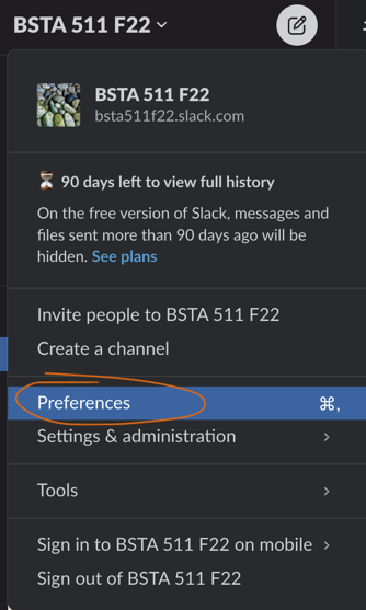
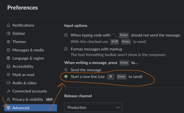
International Day of Women in Statistics and Data Science

Mimi’s tip of the day: sending messages in Slack

Are you frustrated that Slack sends a message when you press Enter? You can change that!

Recap of last time

(1.3) Data collection principles
- Population vs. sample
- Sampling methods
- Experiments vs. Observational studies
(1.2) Intro to Data
- Data types
  - Numerical: discrete (integer in R), continuous (double or numeric in R)
  - Categorical: ordinal, nominal
    - character or factor in R
- How are data stored in R? data frames, tibbles
- Working with data in R: dim(), nrow(), ncol(), names(), str(), summary(), head(), tail(), $
(1.4) Summarizing numerical data
- mean(), median(), sd(), quantile()

R Packages

A good analogy for R packages is that they
are like apps you can download onto a mobile phone:

ModernDive Figure 1.4

From last time: Install the pacakges listed below

knitr
- this might actually already be installed
- check your packages list
tidyverse
- this is actually a bundle of packages
- Warning: it will take a while to install!!!
- see more info at https://tidyverse.tidyverse.org/
rstatix
- for summary statistics of a dataset
janitor
- for cleaning and exploring data
ggridges
- for creating ridgeline plots
devtools
- used to create R packages
- for our purposes, needed to install some packages
oi_biostat_data
- this package is on github
- see the next slide for directions on how to install oi_biostat_data

Directions for installing package `oibiostat`

The textbook’s datasets are in the R package oibiostat
Explanation of code below
- Installation of oibiostat package requires first installing devtools package
- The code devtools::install_github() tells R to use the command install_github() from the devtools package without loading the entire package and all of its commands (which library(devtools) would do).

install.packages("devtools")
devtools::install_github("OI-Biostat/oi_biostat_data", force = TRUE)

After running the code above, put # in front of the commands so that RStudio doesn’t evaluate them when rendering.
Now load the oibiostat package
- the code below needs to be run every time you restart R or render a Qmd file

library(oibiostat)

Load packages with `library()` command

Tip: at the top of your Qmd file, create a chunk that loads all of the R packages you want to use in that file.
Use the library() command to load each required package.
- Packages need to be reloaded every time you open Rstudio.
- library() commands to load needed packages must be in the Qmd file

# run these every time you open Rstudio
library(tidyverse)    
library(oibiostat)
library(ggridges)
library(janitor)
library(rstatix)
library(knitr)
library(gtsummary) # NEW!!

You can check whether a package has been loaded or not
- by looking at the Packages tab and
- seeing whether it has been checked off or not

Case study: discrimination in developmental disability support (Section 1.7.1)

Case Study Description

In the US, individuals with developmental disabilities typically receive services and support from state governments.
- California allocates funds to developmentally disabled residents through the Department of Developmental Services (DDS)
- Recipients of DDS funds are referred to as “consumers.”
Dataset dds.discr
- sample of 1,000 DDS consumers (out of a total of ~ 250,000)
- data include age, gender, race/ethnicity, and annual DDS financial support per consumer
Previous research
- Researchers examined expenditures on consumers by ethnicity
- Found that the mean annual expenditure on Hispanics was less than that on White non-Hispanics.
Result: an allegation of ethnic discrimination was brought against the California DDS.
Question: Are the data sufficient evidence of ethnic discrimination?
See Section 1.7.1 in the textbook for more details

Load `dds.discr` dataset from `oibiostat` package

The textbook’s datasets are in the R package oibiostat
Make sure the oibiostat package is installed before running the code below.
Load the oibiostat package and the dataset dds.discr

the code below needs to be run every time you restart R or render a Qmd file

library(oibiostat)
data("dds.discr")

After loading the dataset dds.discr using data("dds.discr"), you will see dds.discr in the Data list of the Environment window.

Getting to know the dataset

dim(dds.discr)

[1] 1000    6

names(dds.discr)

[1] "id"           "age.cohort"   "age"          "gender"       "expenditures"
[6] "ethnicity"

length(unique(dds.discr$id)) # How many unique id's are there?

[1] 1000

`str()` structure

We previously used the base R structure command str() to get information about variable types in a dataset.
Note this dataset is a tibble instead of a data.frame

str(dds.discr)      # base R

tibble [1,000 × 6] (S3: tbl_df/tbl/data.frame)
 $ id          : int [1:1000] 10210 10409 10486 10538 10568 10690 10711 10778 10820 10823 ...
 $ age.cohort  : Factor w/ 6 levels "0-5","6-12","13-17",..: 3 5 1 4 3 3 3 3 3 3 ...
 $ age         : int [1:1000] 17 37 3 19 13 15 13 17 14 13 ...
 $ gender      : Factor w/ 2 levels "Female","Male": 1 2 2 1 2 1 1 2 1 2 ...
 $ expenditures: int [1:1000] 2113 41924 1454 6400 4412 4566 3915 3873 5021 2887 ...
 $ ethnicity   : Factor w/ 8 levels "American Indian",..: 8 8 4 4 8 4 8 3 8 4 ...
 - attr(*, "spec")=
  .. cols(
  ..   ID = col_integer(),
  ..   `Age Cohort` = col_character(),
  ..   Age = col_integer(),
  ..   Gender = col_character(),
  ..   Expenditures = col_integer(),
  ..   Ethnicity = col_character()
  .. )

`glimpse()`

New: glimpse()

Use glimpse() from the tidyverse package (technically it’s from the dplyr package) to get information about variable types.
glimpse() tends to have nicer output for tibbles than str()

library(tidyverse)
glimpse(dds.discr)  # from tidyverse package (dplyr)

Rows: 1,000
Columns: 6
$ id           <int> 10210, 10409, 10486, 10538, 10568, 10690, 10711, 10778, 1…
$ age.cohort   <fct> 13-17, 22-50, 0-5, 18-21, 13-17, 13-17, 13-17, 13-17, 13-…
$ age          <int> 17, 37, 3, 19, 13, 15, 13, 17, 14, 13, 13, 14, 15, 17, 20…
$ gender       <fct> Female, Male, Male, Female, Male, Female, Female, Male, F…
$ expenditures <int> 2113, 41924, 1454, 6400, 4412, 4566, 3915, 3873, 5021, 28…
$ ethnicity    <fct> White not Hispanic, White not Hispanic, Hispanic, Hispani…

`summary()`

We previously used the base R structure command summary() to get summary information about variables

summary(dds.discr)      # base R

       id        age.cohort       age          gender     expenditures  
 Min.   :10210   0-5  : 82   Min.   : 0.0   Female:503   Min.   :  222  
 1st Qu.:31809   6-12 :175   1st Qu.:12.0   Male  :497   1st Qu.: 2899  
 Median :55384   13-17:212   Median :18.0                Median : 7026  
 Mean   :54663   18-21:199   Mean   :22.8                Mean   :18066  
 3rd Qu.:76135   22-50:226   3rd Qu.:26.0                3rd Qu.:37713  
 Max.   :99898   51+  :106   Max.   :95.0                Max.   :75098  
                                                                        
              ethnicity  
 White not Hispanic:401  
 Hispanic          :376  
 Asian             :129  
 Black             : 59  
 Multi Race        : 26  
 American Indian   :  4  
 (Other)           :  5

`tbl_summary()`: summary table

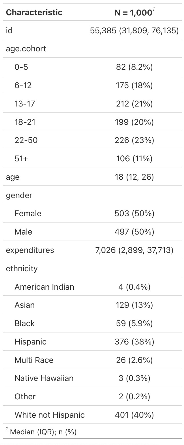
New: Use tbl_summary() from the gtsummary package to get summary information

# library(gtsummary)
tbl_summary(dds.discr)

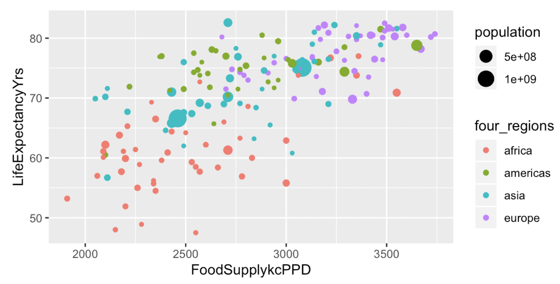
Visualize numerical variables with `ggplot`

What data (variables) are included in the plot below?

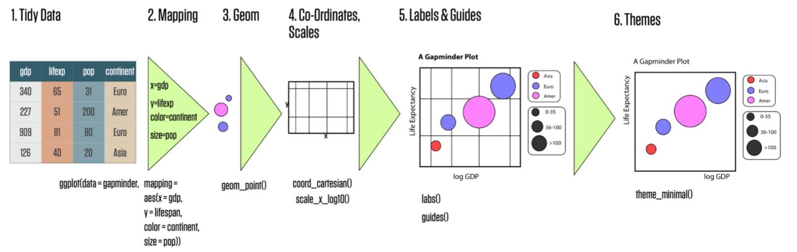
Basics of a ggplot

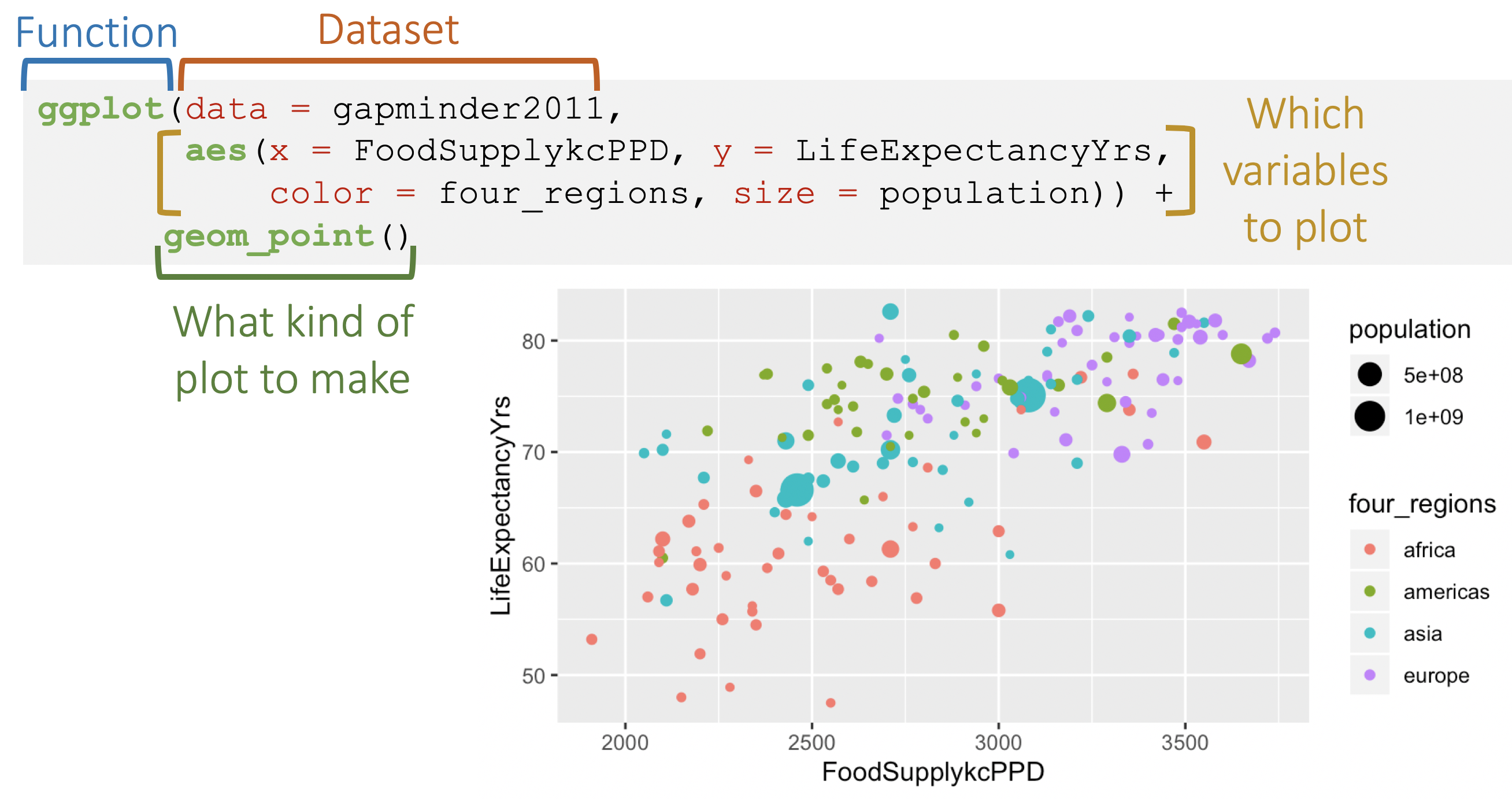
Grammar of ggplot2

Kieran Healy

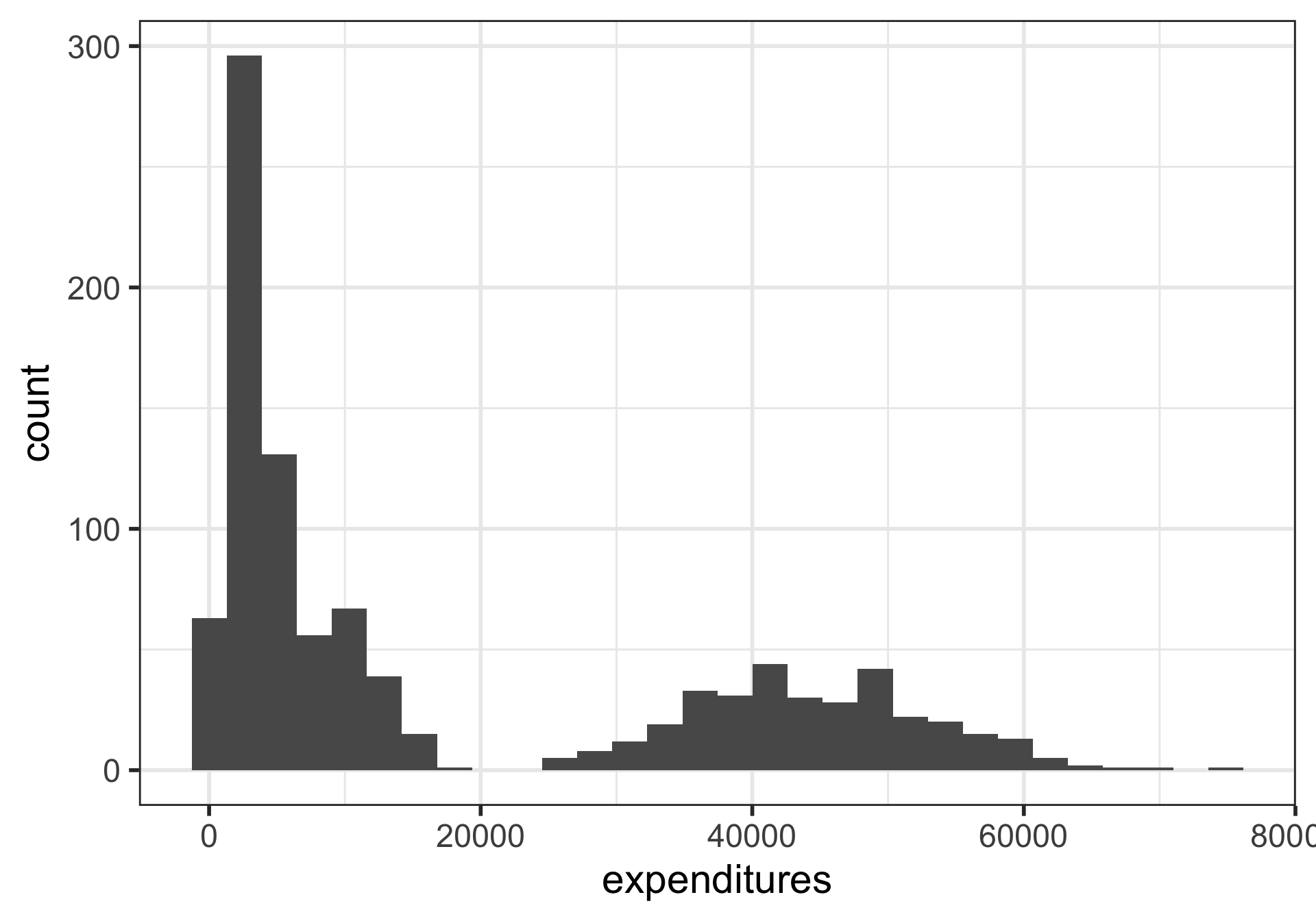
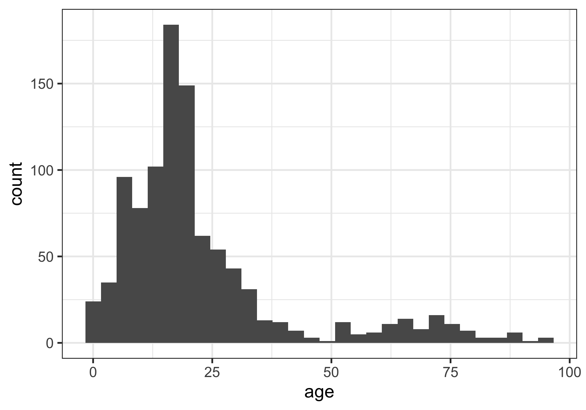
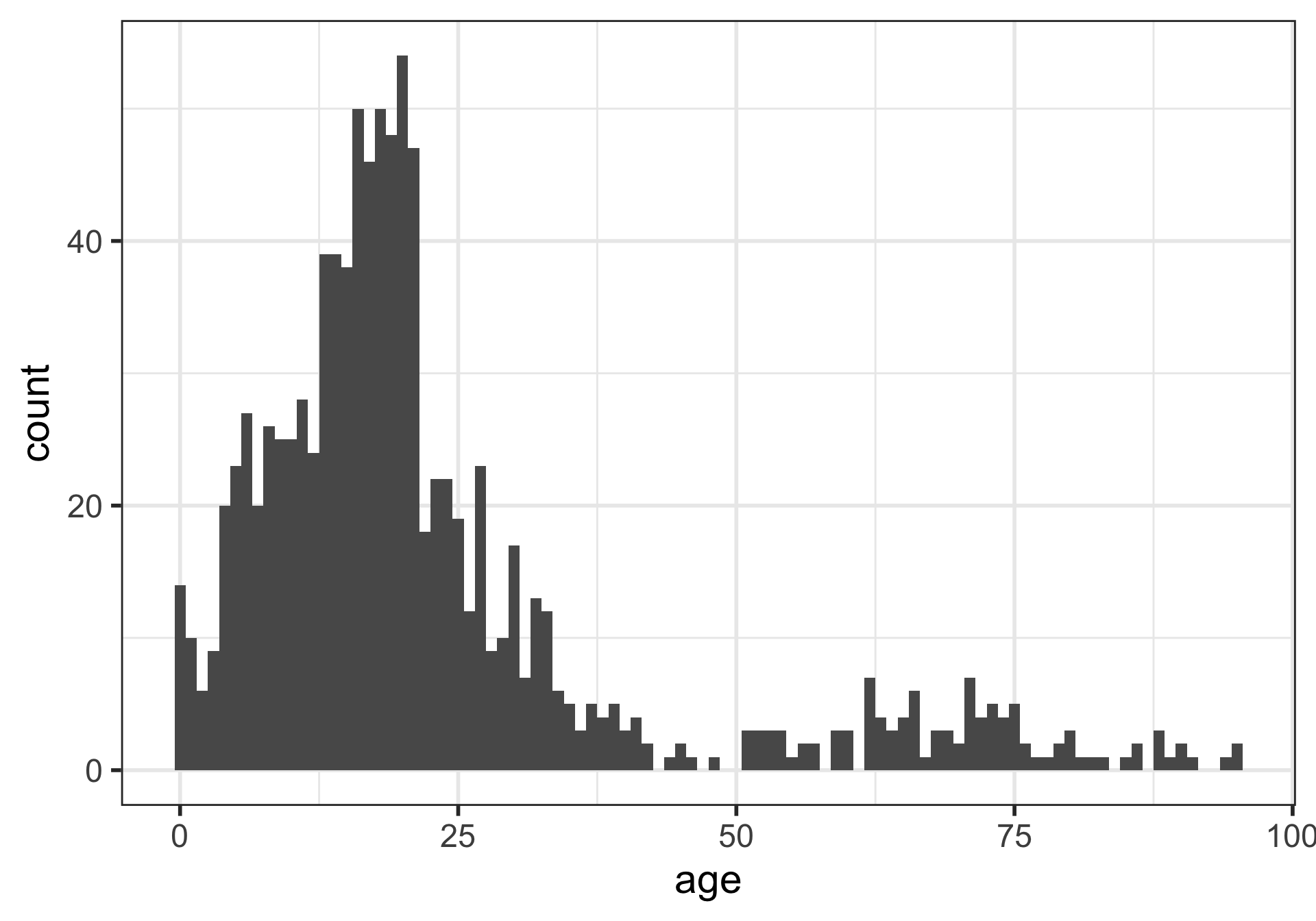
Histograms

What is being measured on the vertical axes?

ggplot(data = dds.discr, 
       aes(x = age)) +
  geom_histogram()

ggplot(data = dds.discr, 
       aes(x = expenditures)) +
  geom_histogram()

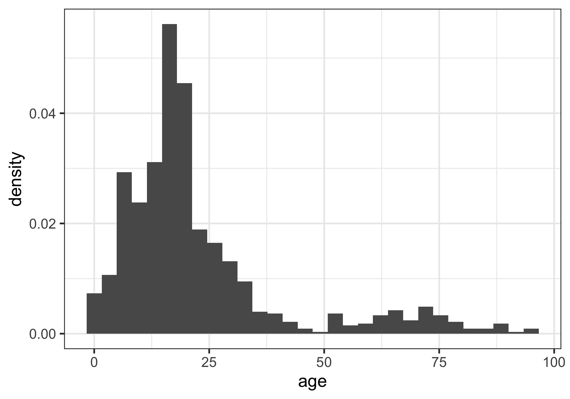
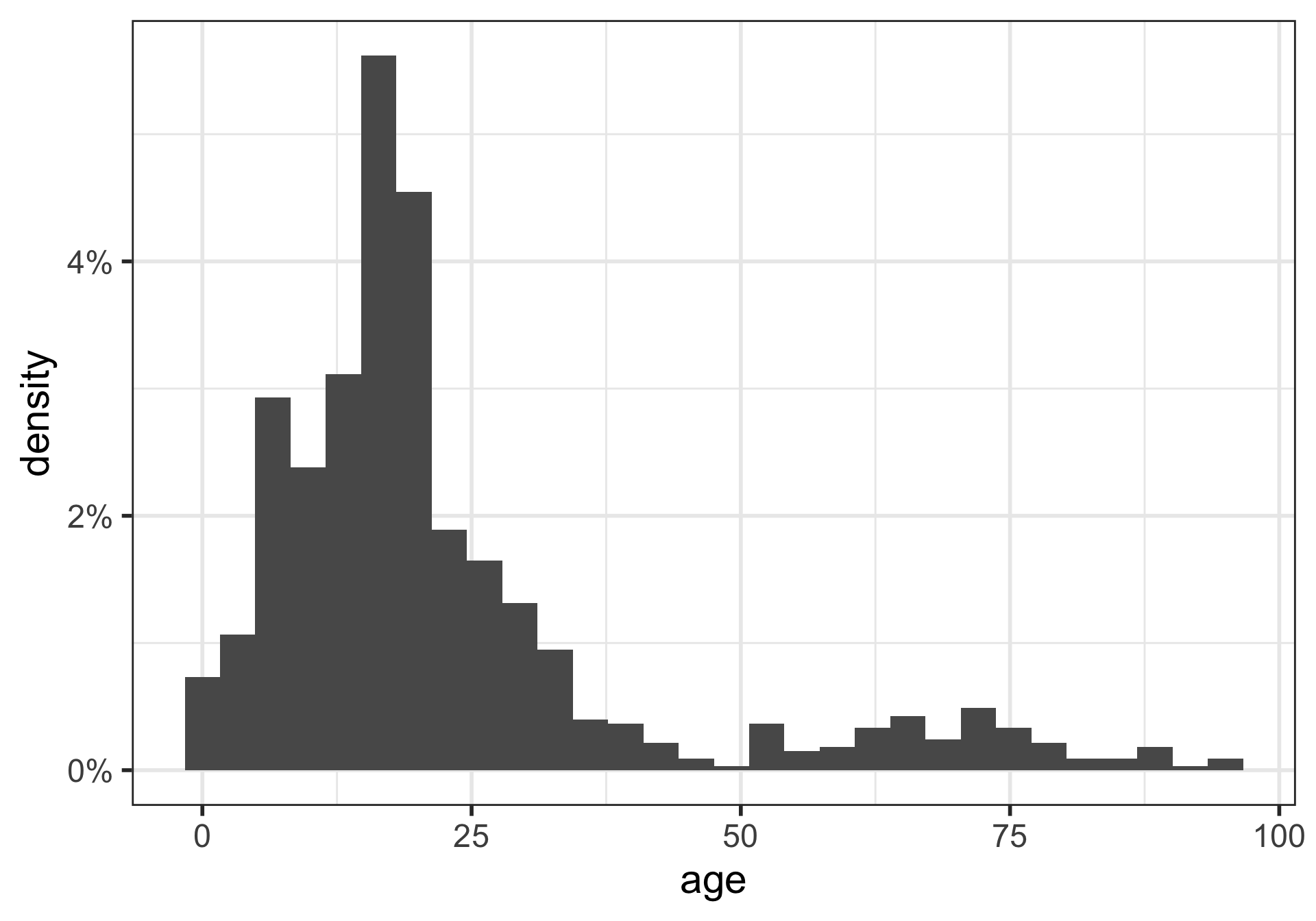
Histograms showing proportions

ggplot(data = dds.discr, 
       aes(x = age)) +
  geom_histogram(
    aes(y = stat(density)))

ggplot(data = dds.discr, 
       aes(x = age)) +
  geom_histogram(
    aes(y = stat(density))) +  
  scale_y_continuous(labels =   
      scales::percent_format())

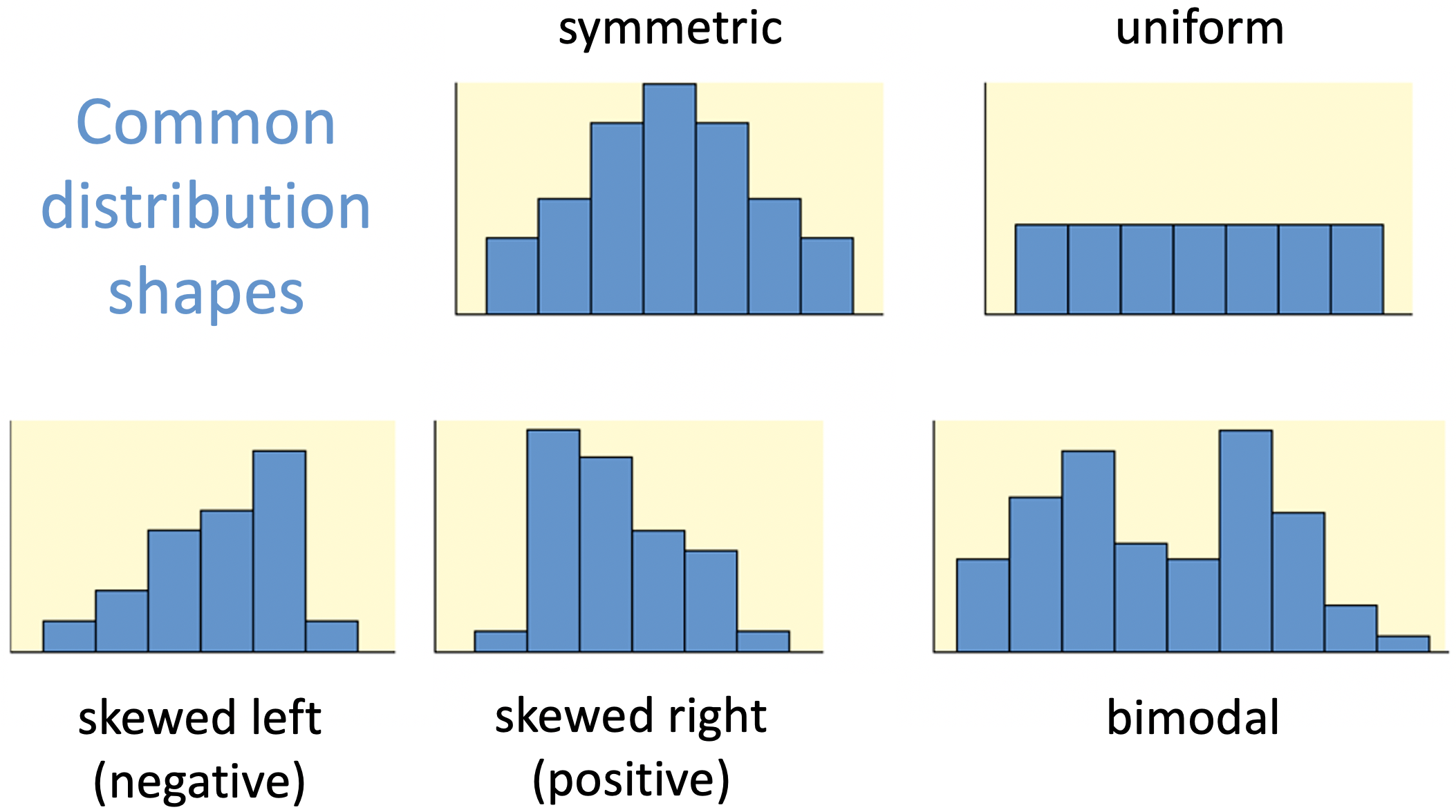
Distribution shapes

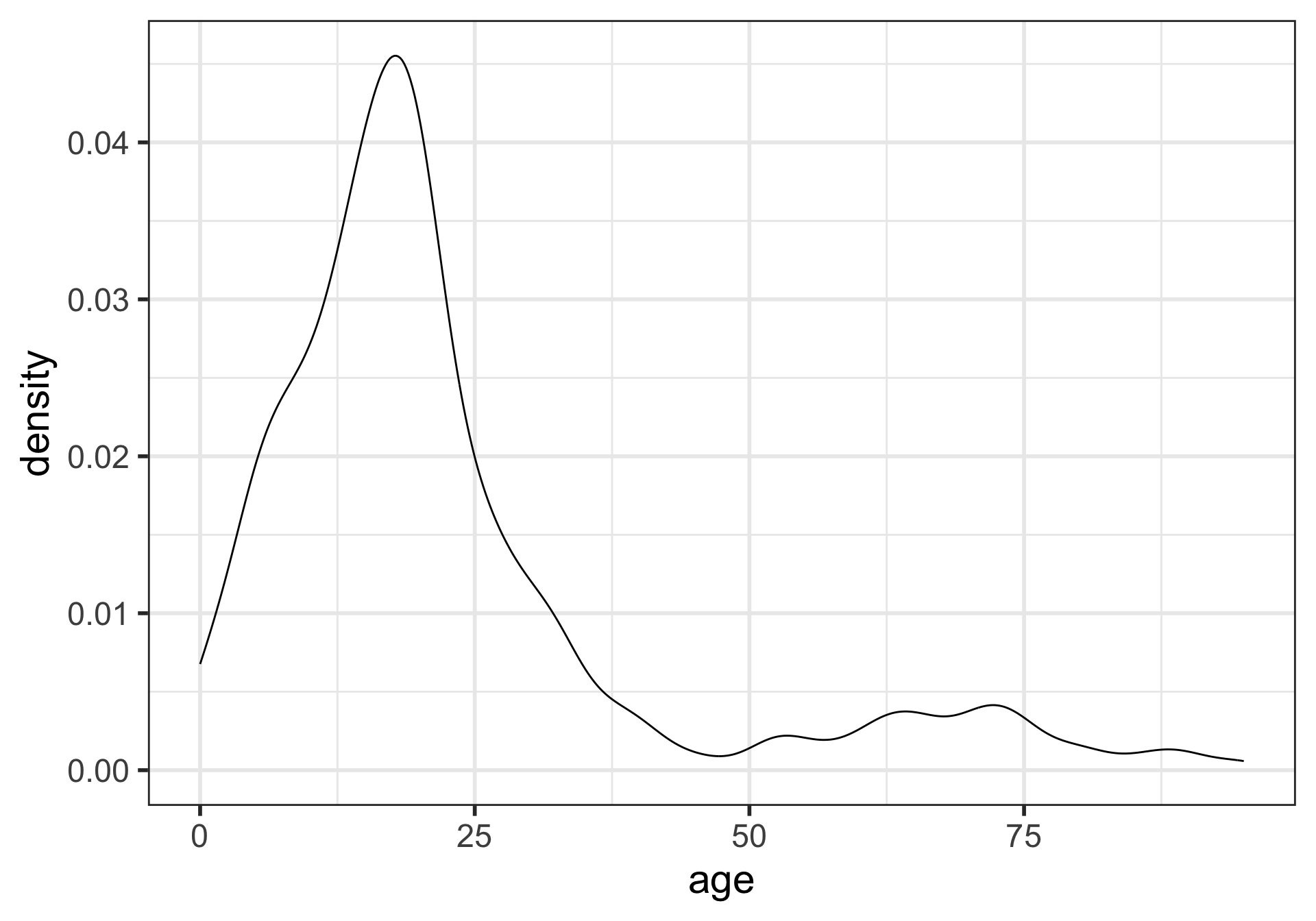
Density plots

What is being measured on the vertical axes?

ggplot(data = dds.discr, 
       aes(x = age)) +
  geom_density()

ggplot(data = dds.discr, 
       aes(x = age)) +
  geom_histogram()

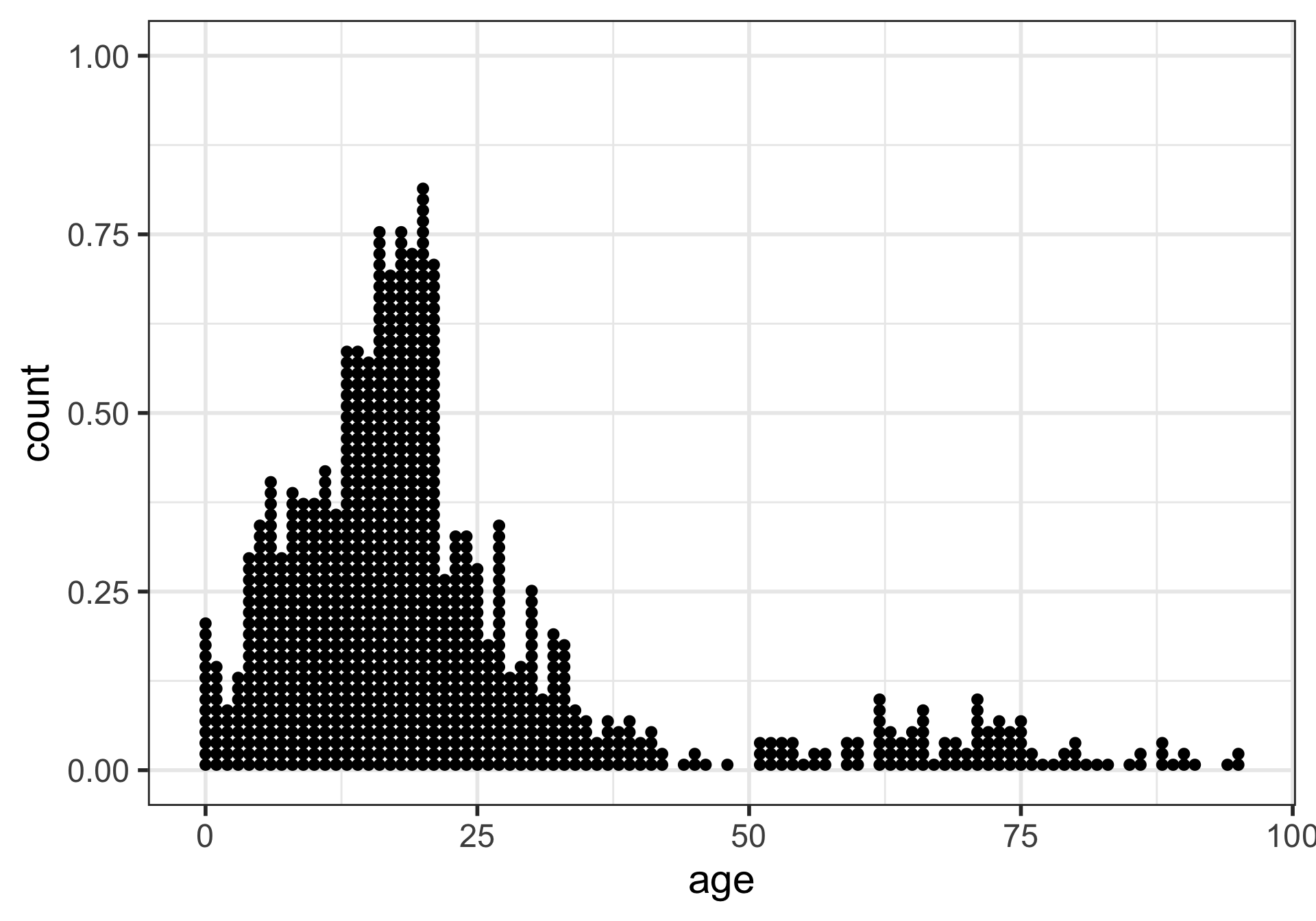
Dot plots

Better for smaller samples
What is being measured on the vertical axes?

ggplot(data = dds.discr, 
       aes(x = age)) +
  geom_dotplot(binwidth =1)

ggplot(data = dds.discr, 
       aes(x = age)) +
  geom_histogram(binwidth =1)

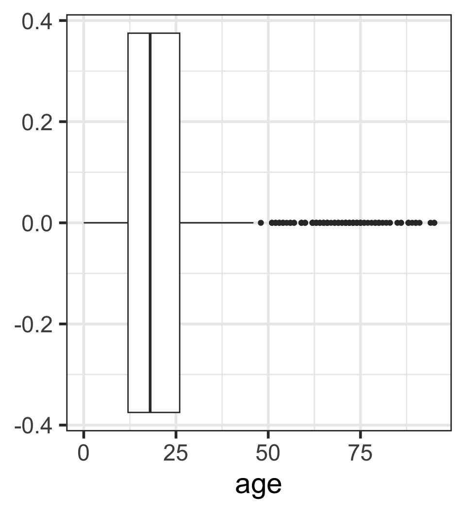
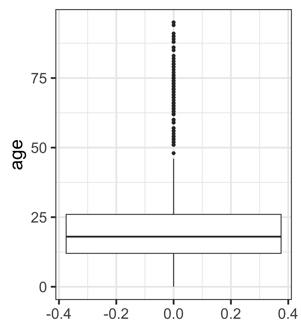
Boxplots

ggplot(data = dds.discr, 
       aes(x = age)) + 
  geom_boxplot()

ggplot(data = dds.discr, 
       aes(y = age)) + 
  geom_boxplot()

Boxplots: 5 number summary visualization

No outliers: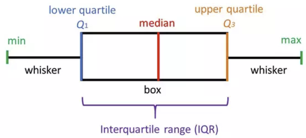

With outliers: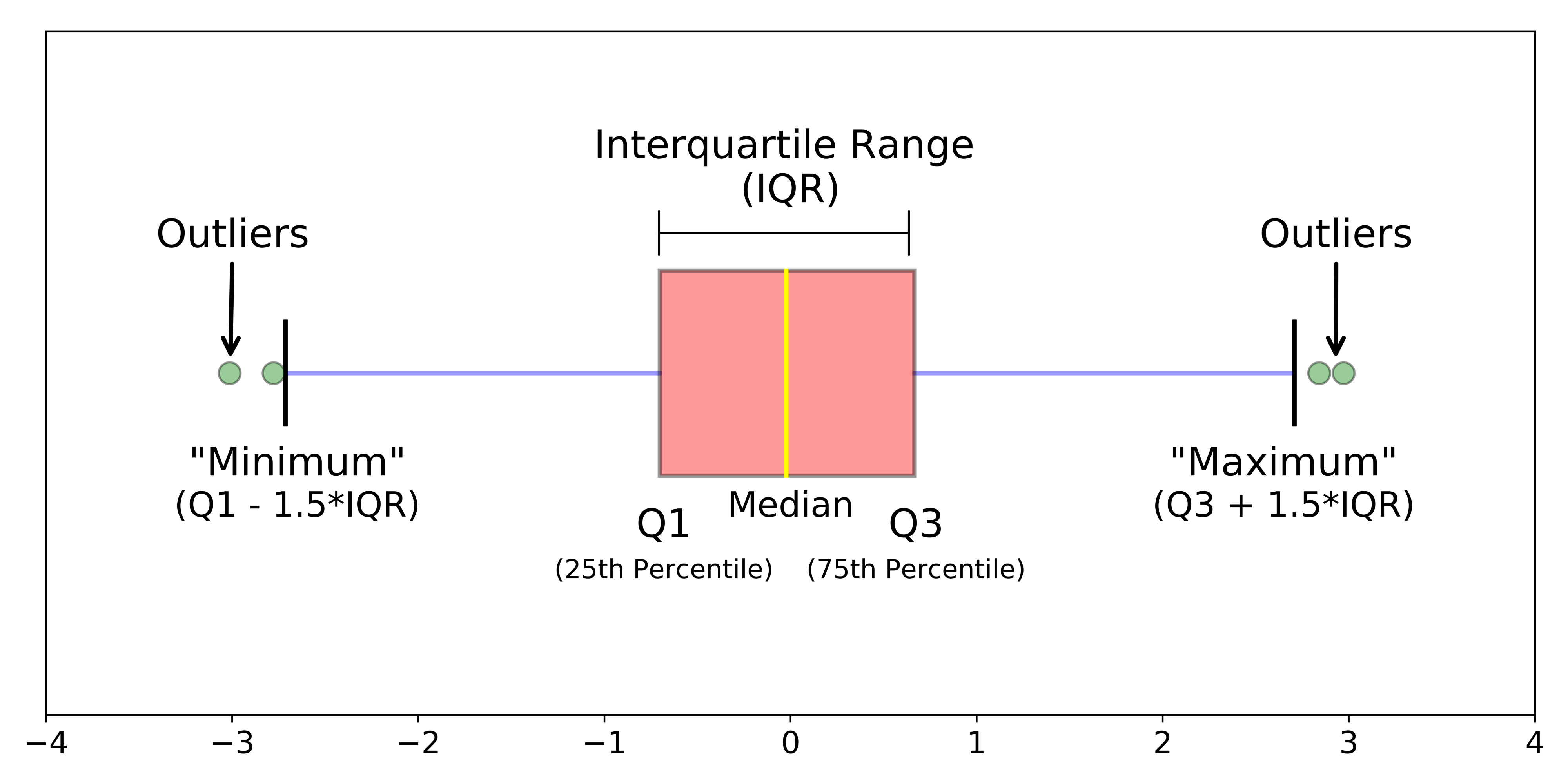

Visualizing relationships between numerical and categorical variables (1.6.3)

Side-by-side boxplots

ggplot(data = dds.discr, 
       aes(x = expenditures,
           y = ethnicity)) + 
  geom_boxplot() + 
  labs(x = "Annual Expenditures ($)", 
       y = "Race and ethnicity")

Can you determine the following using boxplots?

distribution shape
sample size

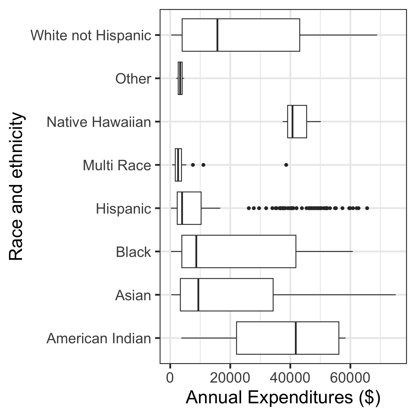
Side-by-side boxplots with data points

ggplot(data = dds.discr, 
       aes(x = expenditures,
           y = ethnicity)) + 
  geom_boxplot(color="darkgrey") + 
  labs(x = "Annual Expenditures ($)",
       y = "Race and ethnicity") +
  geom_jitter(     
    aes(color = ethnicity),      
    alpha = 0.3,      
    show.legend = FALSE,      
    position = position_jitter(     
      height = 0.4))

Can you determine the following using boxplots?

distribution shape
sample size

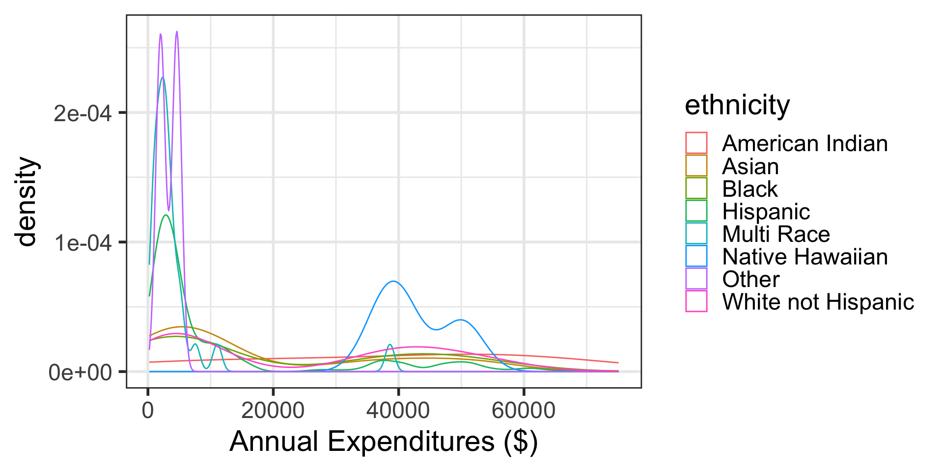
Density plots by group

ggplot(data = dds.discr, 
       aes(x = expenditures,
           color = ethnicity)) + 
  geom_density() + 
  labs(x = "Annual Expenditures ($)")

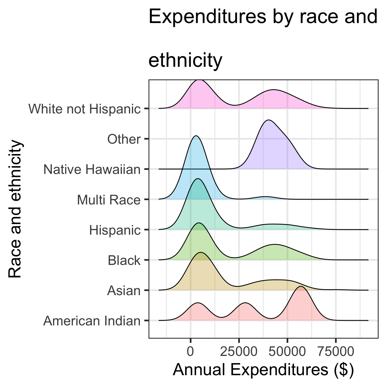
Ridgeline plot

# library(ggridges)
ggplot(data = dds.discr,
       aes(x = expenditures,
           y = ethnicity,      
           fill = ethnicity)      
       ) + 
  geom_density_ridges(      
    alpha = 0.3,      
    show.legend = FALSE) +      
  labs(x = "Annual Expenditures ($)",
       y = "Race and ethnicity",
       title =        
"Expenditures by race and 
       \nethnicity")

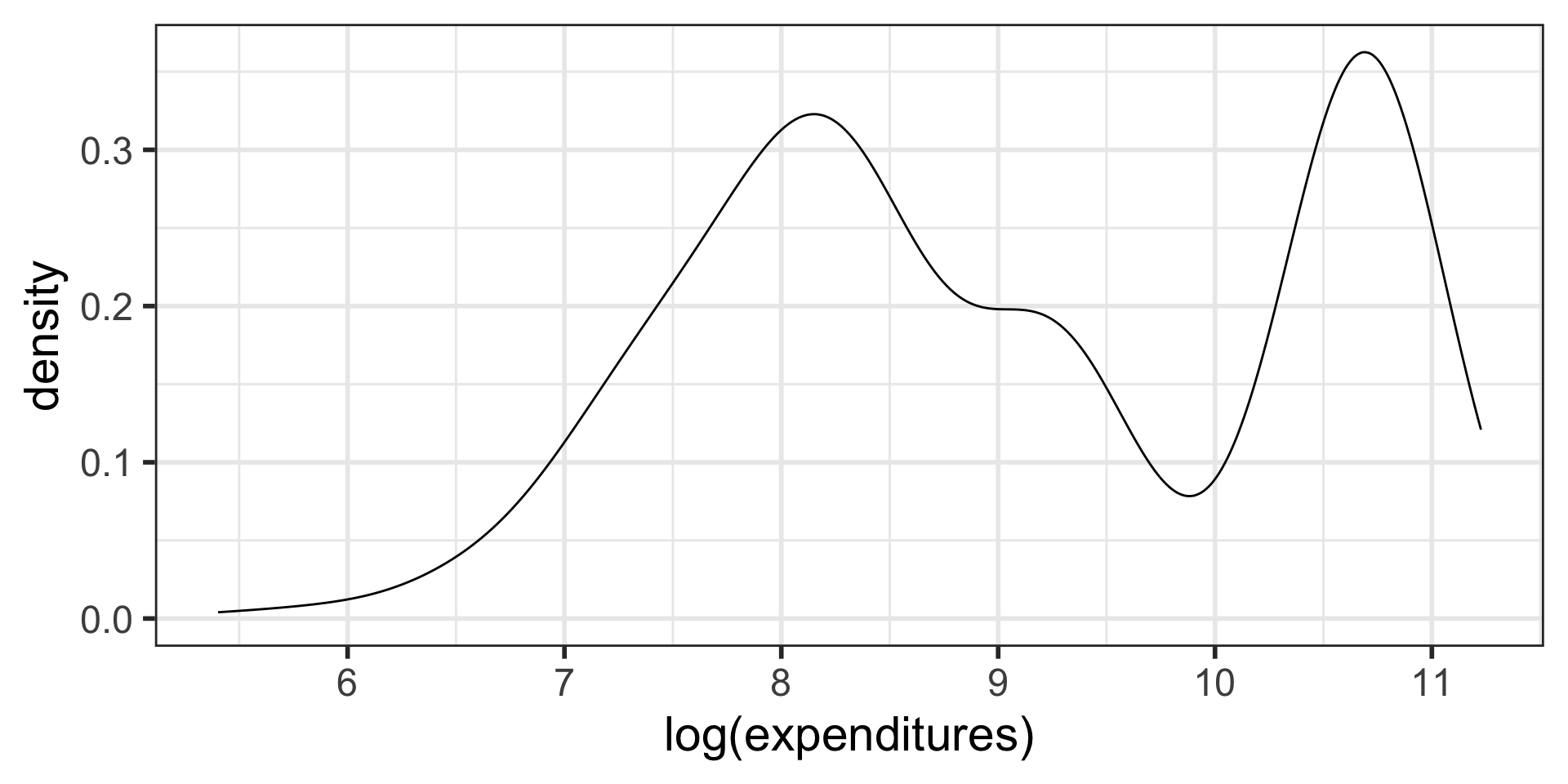
Transforming data (1.4.5)

We sometimes apply a transformation to highly skewed data to make it more symmetric
Log transformations are often used for skewed right data

x = expenditures

ggplot(data = dds.discr, 
       aes(x = expenditures)) +  
  geom_density()

x = log(expenditures)

ggplot(data = dds.discr, 
       aes(x = log(expenditures))) +  
  geom_density()

Relationships between two numerical variables (1.6.1)

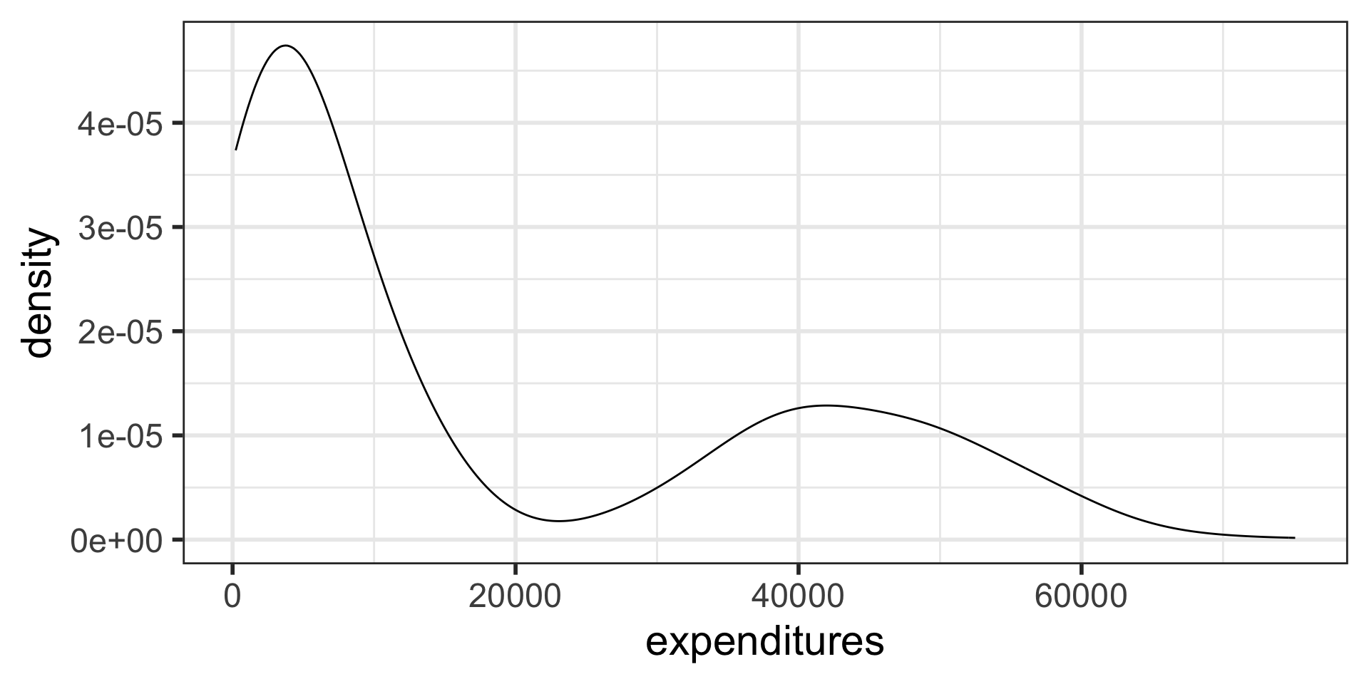
Scatterplots

ggplot(data = dds.discr, 
       aes(x = age,
           y = expenditures)) + 
  geom_point() +       
  labs(x = "Age",
       y = "Annual Expenditures ($)")

Response vs. explanatory variables (Section 1.2.3)

A response variable measures the outcome of interest in a study
A study will typically examine whether the values of a response variable differ as values of an explanatory variable change

Describe the association between the variables

Describing associations between 2 numerical variables

Two variables $x$ and $y$ are

positively associated if $y$ increases as $x$ increases.
negatively associated if $y$ decreases as $x$ increases.
If there is no association between the variables, then we say they are uncorrelated or independent.

The term “association” is a very general term.
- Can be used for numerical or categorical variables
- Not specifically referring to linear associations

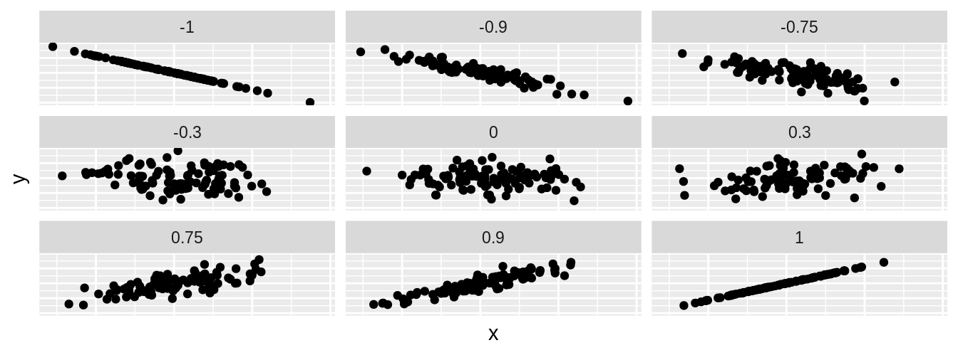
(Pearson) Correlation coefficient $r$

$r = -1$ indicates a perfect negative linear relationship: As one variable increases, the value of the other variable tends to go down, following a straight line.
$r = 0$ indicates no linear relationship: The values of both variables go up/down independently of each other.
$r = 1$ indicates a perfect positive linear relationship: As the value of one variable goes up, the value of the other variable tends to go up as well in a linear fashion.
The closer $r$ is to ±1, the stronger the linear association.

(Pearson) Correlation coefficient (r): formula

The (Peasron) correlation coefficient of variables $x$ and $y$ can be computed using the formula \[r = \frac{1}{n-1}\sum_{i=1}^{n}\Big(\frac{x_i - \bar{x}}{s_x}\Big)\Big(\frac{y_i - \bar{y}}{s_y}\Big)\] where

$(x_1,y_1),(x_2,y_2),...,(x_n,y_n)$ are the $n$ paired values of the variables $x$ and $y$
$s_x$ and $s_y$ are the sample standard deviations of the variables $x$ and $y$, respectively

cor(dds.discr$age, dds.discr$expenditures)

[1] 0.8432422

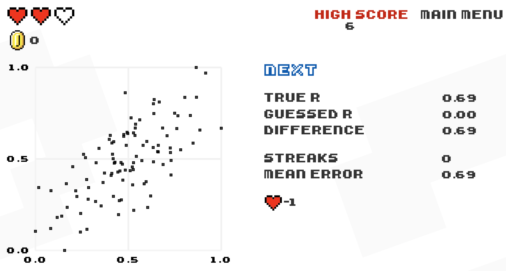
Guess the correlation game!

Rossman & Chance’s applet

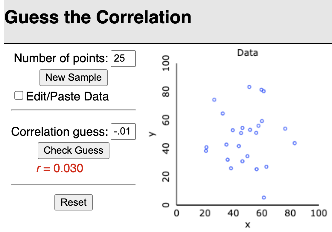
Tracks performance of guess vs. actual, error vs. actual, and error vs. trial

http://www.rossmanchance.com/applets/GuessCorrelation.html

Or, for the Atari-like experience

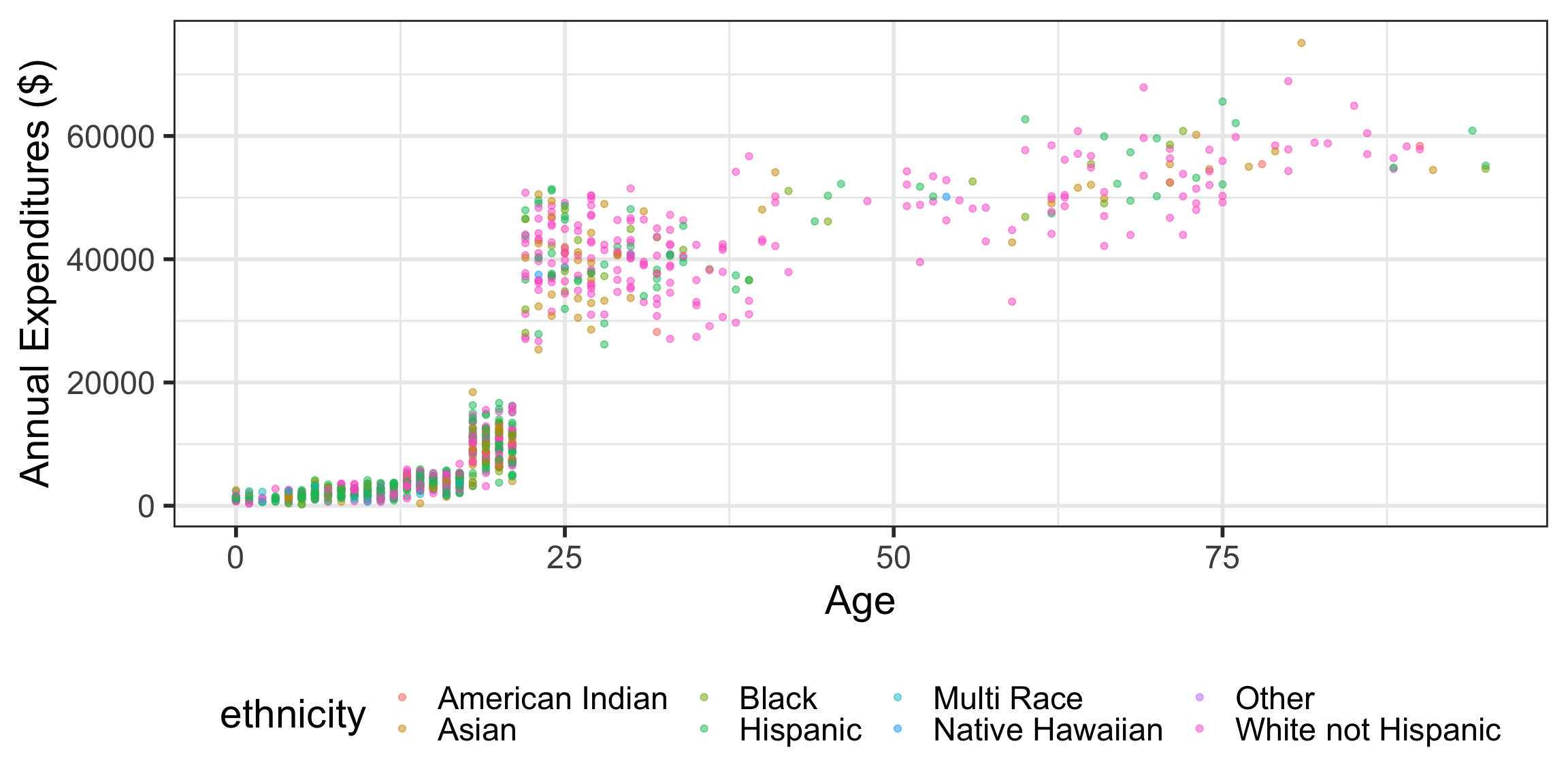
Scatterplots with color-coded dots

Describe the association between the variables

ggplot(data = dds.discr, 
       aes(x = age, y = expenditures,
           color = ethnicity)) +   
  geom_point(alpha = .5) +       
  labs(x = "Age", y = "Annual Expenditures ($)") +
  theme(legend.position = "bottom")

Categorical data (1.5) and Relationships between two categorical variables (1.6.2)

Barplots

Counts (below) vs.
percentages (right)

ggplot(data = dds.discr, 
       aes(x = ethnicity)) +
  geom_bar()

ggplot(data = dds.discr, 
       aes(x = ethnicity)) +
  geom_bar(aes(y = stat(prop),  
               group = 1)) + 
  scale_y_continuous(labels =  
      scales::percent_format())

Barplots with 2 variables: segmented bar plots

ggplot(data = dds.discr, 
       aes(x = ethnicity,
           fill = age.cohort)) + 
  geom_bar()

ggplot(data = dds.discr, 
       aes(x = ethnicity,
           fill = age.cohort)) + 
  geom_bar(position = "fill")

Summarizing categorical data and some data wrangling

Frequency tables: `count()`

count is from the dplyr package
the output is a long tibble, and not a “nice” table

dds.discr %>% count(ethnicity)

# A tibble: 8 × 2
  ethnicity              n
  <fct>              <int>
1 American Indian        4
2 Asian                129
3 Black                 59
4 Hispanic             376
5 Multi Race            26
6 Native Hawaiian        3
7 Other                  2
8 White not Hispanic   401

dds.discr %>% 
  count(ethnicity, age.cohort)

# A tibble: 35 × 3
   ethnicity       age.cohort     n
   <fct>           <fct>      <int>
 1 American Indian 13-17          1
 2 American Indian 22-50          1
 3 American Indian 51+            2
 4 Asian           0-5            8
 5 Asian           6-12          18
 6 Asian           13-17         20
 7 Asian           18-21         41
 8 Asian           22-50         29
 9 Asian           51+           13
10 Black           0-5            3
# ℹ 25 more rows

How to use the pipe `%>%`

The pipe operator %>% strings together commands to be performed sequentially

dds.discr %>% head(n=3)      # pronounce %>% as "then"

# A tibble: 3 × 6
     id age.cohort   age gender expenditures ethnicity         
  <int> <fct>      <int> <fct>         <int> <fct>             
1 10210 13-17         17 Female         2113 White not Hispanic
2 10409 22-50         37 Male          41924 White not Hispanic
3 10486 0-5            3 Male           1454 Hispanic

Always first list the tibble that the commands are being applied to
Can use multiple pipes to run multiple commands in sequence
- What does the following code do?

dds.discr %>% head(n=3) %>% summary()

Frequency tables: `janitor` package’s `tabyl` function

# default table
dds.discr %>% 
  tabyl(ethnicity)

          ethnicity   n percent
    American Indian   4   0.004
              Asian 129   0.129
              Black  59   0.059
           Hispanic 376   0.376
         Multi Race  26   0.026
    Native Hawaiian   3   0.003
              Other   2   0.002
 White not Hispanic 401   0.401

adorn_ your table!

dds.discr %>% 
  tabyl(ethnicity) %>%
  adorn_totals("row") %>% 
  adorn_pct_formatting(digits=2)

          ethnicity    n percent
    American Indian    4   0.40%
              Asian  129  12.90%
              Black   59   5.90%
           Hispanic  376  37.60%
         Multi Race   26   2.60%
    Native Hawaiian    3   0.30%
              Other    2   0.20%
 White not Hispanic  401  40.10%
              Total 1000 100.00%

Relative frequency table

A relative frequency table shows proportions (or percentages) instead of counts
To the right I removed (deselected) the counts column (n) to create a relative frequency table

dds.discr %>% 
  tabyl(ethnicity) %>%
  adorn_totals("row") %>% 
  adorn_pct_formatting(digits=2) %>%   
  select(-n)

          ethnicity percent
    American Indian   0.40%
              Asian  12.90%
              Black   5.90%
           Hispanic  37.60%
         Multi Race   2.60%
    Native Hawaiian   0.30%
              Other   0.20%
 White not Hispanic  40.10%
              Total 100.00%

Contingency tables (two-way tables)

Contingency tables summarize data for two categorical variables
- with each value in the table representing the number of times
  a particular combination of outcomes occurs
Row & column totals
are sometimes called marginal totals

dds.discr %>% 
  tabyl(ethnicity, gender) %>%    
  adorn_totals(c("row", "col"))

          ethnicity Female Male Total
    American Indian      3    1     4
              Asian     61   68   129
              Black     26   33    59
           Hispanic    192  184   376
         Multi Race     13   13    26
    Native Hawaiian      2    1     3
              Other      1    1     2
 White not Hispanic    205  196   401
              Total    503  497  1000

Contingency tables with percentages

dds.discr %>% 
  tabyl(ethnicity, age.cohort) %>%
  adorn_totals(c("row")) %>%
  adorn_percentages("row") %>%   
  adorn_pct_formatting(digits=0) %>%    
  adorn_ns()

          ethnicity      0-5      6-12      13-17     18-21     22-50       51+
    American Indian  0%  (0)  0%   (0)  25%   (1)  0%   (0) 25%   (1) 50%   (2)
              Asian  6%  (8) 14%  (18)  16%  (20) 32%  (41) 22%  (29) 10%  (13)
              Black  5%  (3) 19%  (11)  20%  (12) 15%   (9) 29%  (17) 12%   (7)
           Hispanic 12% (44) 24%  (91)  27% (103) 21%  (78) 11%  (43)  5%  (17)
         Multi Race 27%  (7) 35%   (9)  27%   (7)  8%   (2)  4%   (1)  0%   (0)
    Native Hawaiian  0%  (0)  0%   (0)   0%   (0)  0%   (0) 67%   (2) 33%   (1)
              Other  0%  (0)  0%   (0) 100%   (2)  0%   (0)  0%   (0)  0%   (0)
 White not Hispanic  5% (20) 11%  (46)  17%  (67) 17%  (69) 33% (133) 16%  (66)
              Total  8% (82) 18% (175)  21% (212) 20% (199) 23% (226) 11% (106)

Summarizing numeric data

Mean annual DDS expenditures by race/ethnicity

mean(dds.discr$expenditures)

[1] 18065.79

dds.discr %>% 
  summarize(
    ave = mean(expenditures),
    SD = sd(expenditures),
    med = median(expenditures))

# A tibble: 1 × 3
     ave     SD   med
   <dbl>  <dbl> <dbl>
1 18066. 19543.  7026

dds.discr %>% 
  group_by(ethnicity) %>% 
  summarize(
    ave = mean(expenditures),
    SD = sd(expenditures),
    med = median(expenditures))

# A tibble: 8 × 4
  ethnicity             ave     SD    med
  <fct>               <dbl>  <dbl>  <dbl>
1 American Indian    36438. 25694. 41818.
2 Asian              18392. 19209.  9369 
3 Black              20885. 20549.  8687 
4 Hispanic           11066. 15630.  3952 
5 Multi Race          4457.  7332.  2622 
6 Native Hawaiian    42782.  6576. 40727 
7 Other               3316.  1836.  3316.
8 White not Hispanic 24698. 20604. 15718

`get_summary_stats()` from `rstatix` package

dds.discr %>% get_summary_stats()

# A tibble: 3 × 13
  variable         n   min   max median     q1     q3   iqr    mad   mean     sd
  <fct>        <dbl> <dbl> <dbl>  <dbl>  <dbl>  <dbl> <dbl>  <dbl>  <dbl>  <dbl>
1 id            1000 10210 99898 55384. 31809. 76135. 44326 3.27e4 5.47e4 2.56e4
2 age           1000     0    95    18     12     26     14 1.04e1 2.28e1 1.85e1
3 expenditures  1000   222 75098  7026   2899. 37713. 34814 7.76e3 1.81e4 1.95e4
# ℹ 2 more variables: se <dbl>, ci <dbl>

dds.discr %>% 
  group_by(ethnicity) %>%
  get_summary_stats(expenditures, type = "common")

# A tibble: 8 × 11
  ethnicity variable     n   min   max median    iqr   mean     sd     se     ci
  <fct>     <fct>    <dbl> <dbl> <dbl>  <dbl>  <dbl>  <dbl>  <dbl>  <dbl>  <dbl>
1 American… expendi…     4  3726 58392 41818. 34085. 36438. 25694. 12847. 40885.
2 Asian     expendi…   129   374 75098  9369  30892  18392. 19209.  1691.  3346.
3 Black     expendi…    59   240 60808  8687  37987  20885. 20549.  2675.  5355.
4 Hispanic  expendi…   376   222 65581  3952   7961. 11066. 15630.   806.  1585.
5 Multi Ra… expendi…    26   669 38619  2622   2060.  4457.  7332.  1438.  2962.
6 Native H… expendi…     3 37479 50141 40727   6331  42782.  6576.  3797. 16337.
7 Other     expendi…     2  2018  4615  3316.  1298.  3316.  1836.  1298. 16499.
8 White no… expendi…   401   340 68890 15718  39157  24698. 20604.  1029.  2023.

How to force all output to be shown? (1/2)

Use kable() from the knitr package.

dds.discr %>% get_summary_stats() %>% kable()

variable	n	min	max	median	q1	q3	iqr	mad	mean	sd	se	ci
id	1000	10210	99898	55384.5	31808.75	76134.75	44326	32734.325	54662.85	25643.673	810.924	1591.310
age	1000	0	95	18.0	12.00	26.00	14	10.378	22.80	18.462	0.584	1.146
expenditures	1000	222	75098	7026.0	2898.75	37712.75	34814	7760.670	18065.79	19542.831	617.999	1212.724

How to force all output to be shown? `knitr` (2/2)

Use kable() from the knitr package.

dds.discr %>% 
  group_by(ethnicity) %>%
  get_summary_stats(expenditures, type = "common") %>% 
  kable()

ethnicity	variable	n	min	max	median	iqr	mean	sd	se	ci
American Indian	expenditures	4	3726	58392	41817.5	34085.25	36438.250	25693.912	12846.956	40884.748
Asian	expenditures	129	374	75098	9369.0	30892.00	18392.372	19209.225	1691.278	3346.482
Black	expenditures	59	240	60808	8687.0	37987.00	20884.593	20549.274	2675.288	5355.170
Hispanic	expenditures	376	222	65581	3952.0	7961.25	11065.569	15629.847	806.048	1584.940
Multi Race	expenditures	26	669	38619	2622.0	2059.75	4456.731	7332.135	1437.950	2961.514
Native Hawaiian	expenditures	3	37479	50141	40727.0	6331.00	42782.333	6576.462	3796.922	16336.838
Other	expenditures	2	2018	4615	3316.5	1298.50	3316.500	1836.356	1298.500	16499.007
White not Hispanic	expenditures	401	340	68890	15718.0	39157.00	24697.549	20604.376	1028.933	2022.793

Back to research question

Case study: discrimination in developmental disability support (1.7.1)

Previous research
- Researchers examined DDS expenditures for developmentally disabled residents by ethnicity
- Found that the mean annual expenditures on Hispanics was less than that on White non-Hispanics.
Result: an allegation of ethnic discrimination was brought against the California DDS.
Question: Are the data sufficient evidence of ethnic discrimination?

Day 3: Data visualization

Goals for today

International Day of Women in Statistics and Data Science

Mimi’s tip of the day: sending messages in Slack

Recap of last time

R Packages

From last time: Install the pacakges listed below

Directions for installing package oibiostat

Load packages with library() command

Case study: discrimination in developmental disability support (Section 1.7.1)

Case Study Description

Load dds.discr dataset from oibiostat package

Getting to know the dataset

str() structure

glimpse()

summary()

tbl_summary(): summary table

Visualize numerical variables with ggplot

What data (variables) are included in the plot below?

Basics of a ggplot

Grammar of ggplot2

Histograms

Histograms showing proportions

Distribution shapes

Density plots

Dot plots

Boxplots

Boxplots: 5 number summary visualization

Visualizing relationships between numerical and categorical variables (1.6.3)

Side-by-side boxplots

Side-by-side boxplots with data points

Density plots by group

Ridgeline plot

Transforming data (1.4.5)

Relationships between two numerical variables (1.6.1)

Scatterplots

Describing associations between 2 numerical variables

(Pearson) Correlation coefficient \(r\)

(Pearson) Correlation coefficient (r): formula

Guess the correlation game!

Scatterplots with color-coded dots

Categorical data (1.5) and Relationships between two categorical variables (1.6.2)

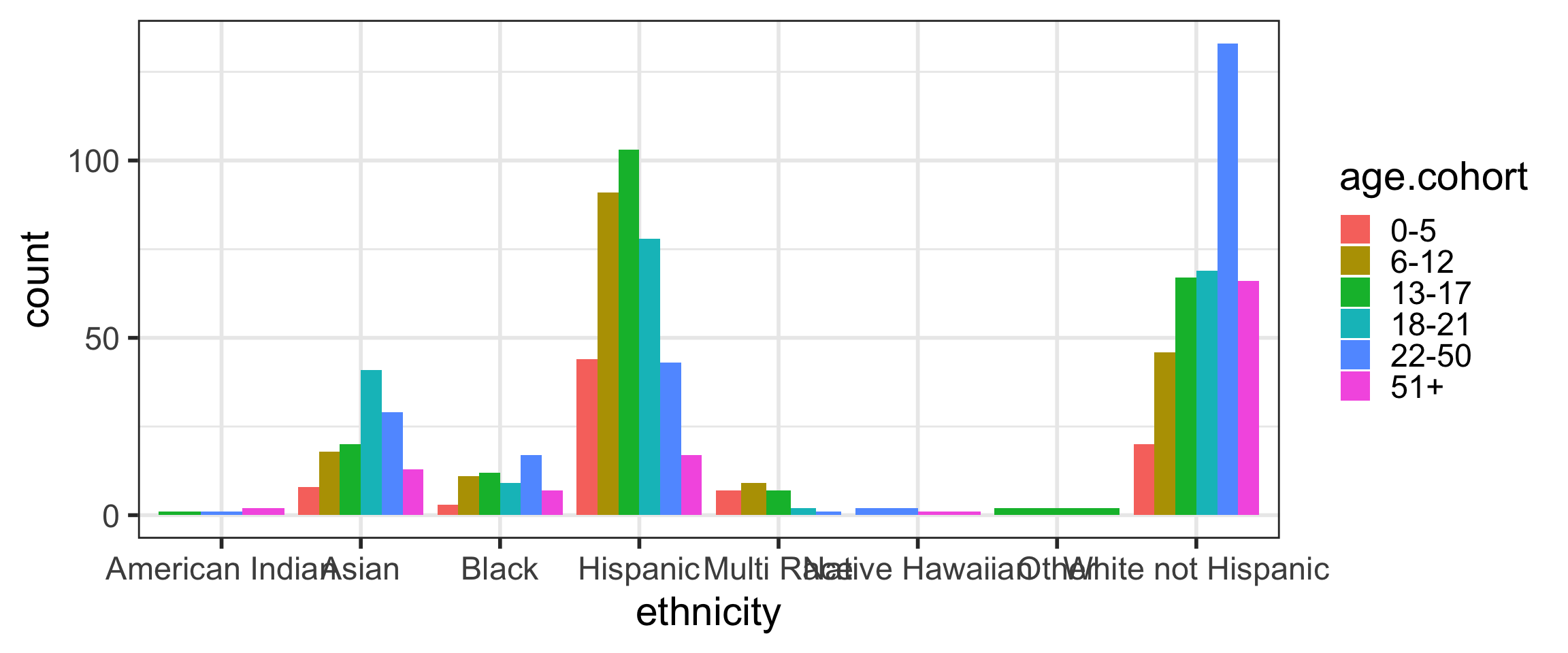
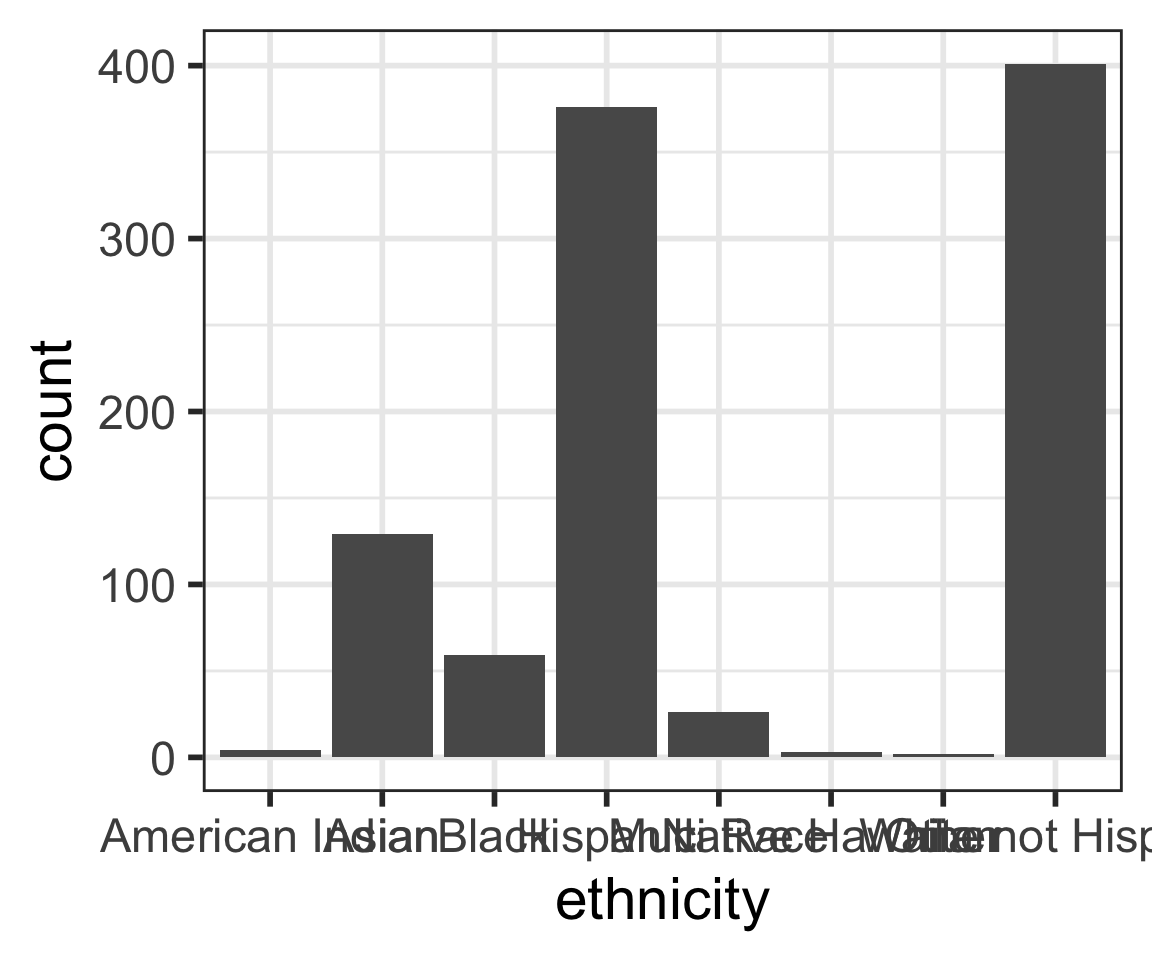
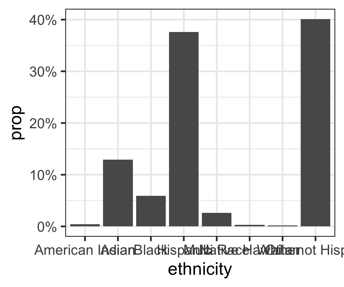
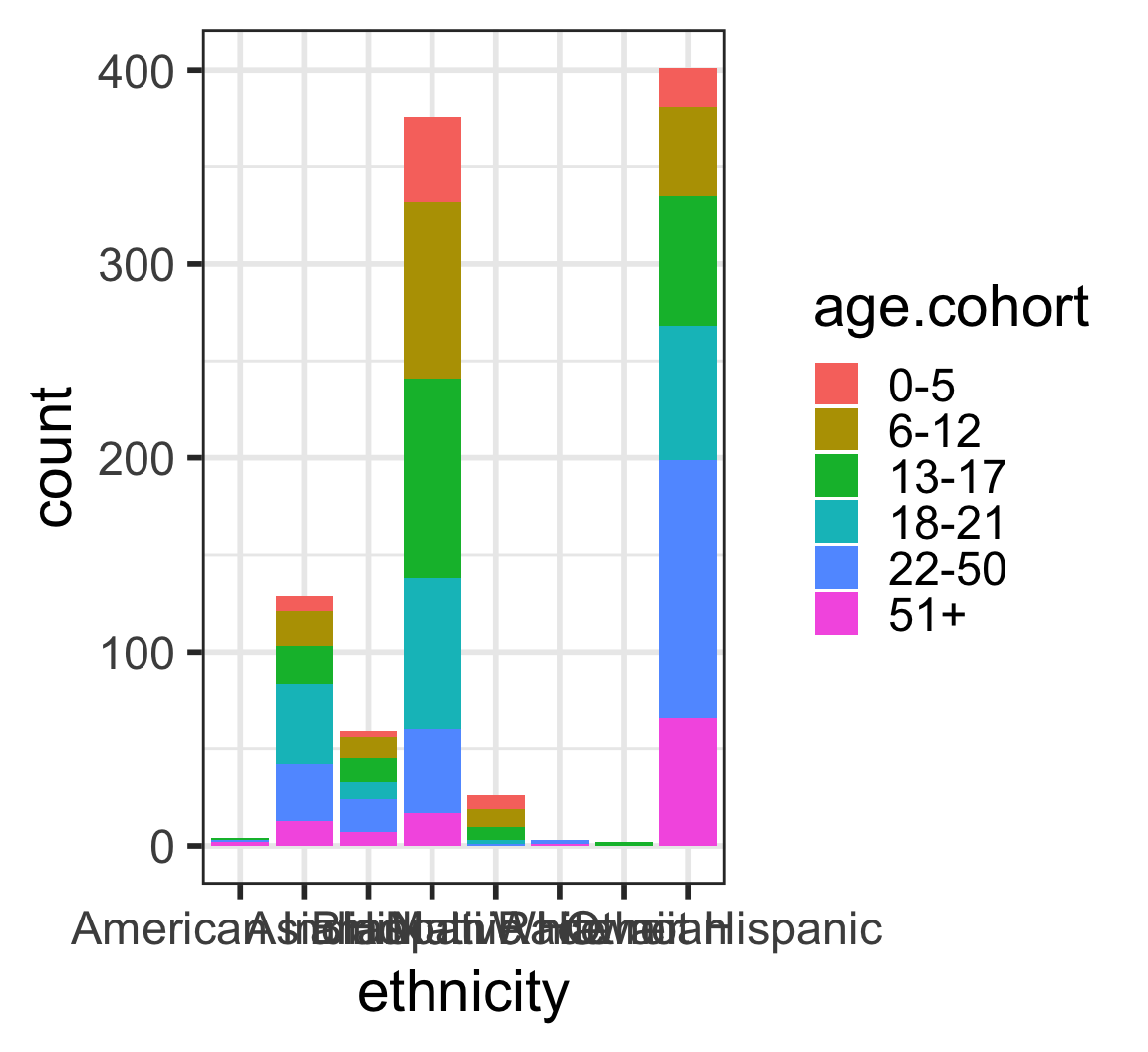
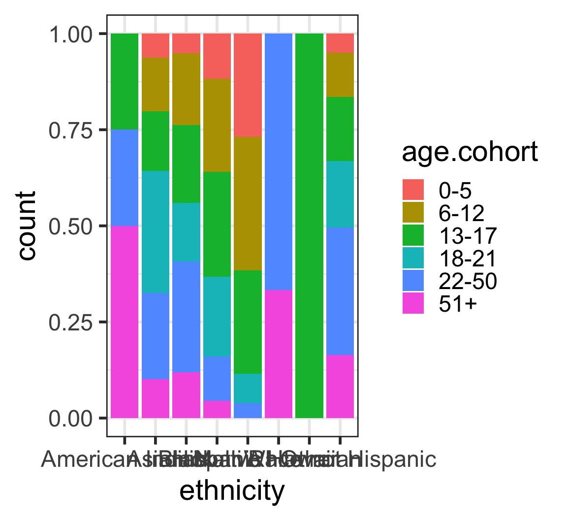
Barplots

Barplots with 2 variables: segmented bar plots

Barplots with 2 variables: side-by-side bar plots

Summarizing categorical data and some data wrangling

Frequency tables: count()

How to use the pipe %>%

Frequency tables: janitor package’s tabyl function

Relative frequency table

Contingency tables (two-way tables)

Contingency tables with percentages

Summarizing numeric data

Mean annual DDS expenditures by race/ethnicity

get_summary_stats() from rstatix package

How to force all output to be shown? (1/2)

How to force all output to be shown? knitr (2/2)

Back to research question

Case study: discrimination in developmental disability support (1.7.1)

Directions for installing package `oibiostat`

Load packages with `library()` command

Load `dds.discr` dataset from `oibiostat` package

`str()` structure

`glimpse()`

`summary()`

`tbl_summary()`: summary table

Visualize numerical variables with `ggplot`

Frequency tables: `count()`

How to use the pipe `%>%`

Frequency tables: `janitor` package’s `tabyl` function

`get_summary_stats()` from `rstatix` package

How to force all output to be shown? `knitr` (2/2)