Day 3 code: Data visualization

BSTA 511/611, OHSU

Week 2

Author

Meike Niederhausen, PhD

Published

October 4, 2023

Back to research question

Case study: discrimination in developmental disability support (1.7.1)

Previous research
- Researchers examined DDS expenditures for developmentally disabled residents by ethnicity
- Found that the mean annual expenditures on Hispanics was less than that on White non-Hispanics.
Result: an allegation of ethnic discrimination was brought against the California DDS.
Question: Are the data sufficient evidence of ethnic discrimination?

Load `dds.discr` dataset from `oibiostat` package

The textbook’s datasets are in the R package oibiostat
Make sure the oibiostat package is installed before running the code below.
Load the oibiostat package and the dataset dds.discr

the code below needs to be run every time you restart R or render a Qmd file

library(oibiostat)
data("dds.discr")

After loading the dataset dds.discr using data("dds.discr"), you will see dds.discr in the Data list of the Environment window.

`glimpse()`

New: glimpse()

Use glimpse() from the tidyverse package (technically it’s from the dplyr package) to get information about variable types.
glimpse() tends to have nicer output for tibbles than str()

library(tidyverse)
glimpse(dds.discr)  # from tidyverse package (dplyr)

Rows: 1,000
Columns: 6
$ id           <int> 10210, 10409, 10486, 10538, 10568, 10690, 10711, 10778, 1…
$ age.cohort   <fct> 13-17, 22-50, 0-5, 18-21, 13-17, 13-17, 13-17, 13-17, 13-…
$ age          <int> 17, 37, 3, 19, 13, 15, 13, 17, 14, 13, 13, 14, 15, 17, 20…
$ gender       <fct> Female, Male, Male, Female, Male, Female, Female, Male, F…
$ expenditures <int> 2113, 41924, 1454, 6400, 4412, 4566, 3915, 3873, 5021, 28…
$ ethnicity    <fct> White not Hispanic, White not Hispanic, Hispanic, Hispani…

Recall previous data viz

ggplot(data = dds.discr, 
       aes(x = expenditures,
           y = ethnicity)) + 
  geom_boxplot(color="darkgrey") + 
  labs(x = "Annual Expenditures ($)",
       y = "Race and ethnicity") +
  geom_jitter(     
    aes(color = ethnicity),      
    alpha = 0.3,      
    show.legend = FALSE,      
    position = position_jitter(height = 0.4))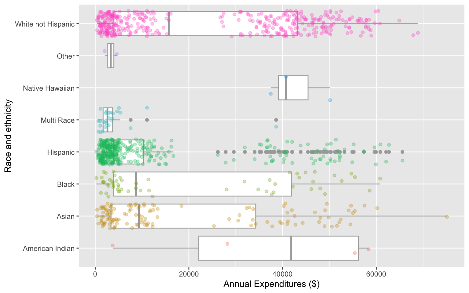

ggplot(data = dds.discr, 
       aes(x = age,
           y = expenditures)) + 
  geom_point() +       
  labs(x = "Age",
       y = "Annual Expenditures ($)")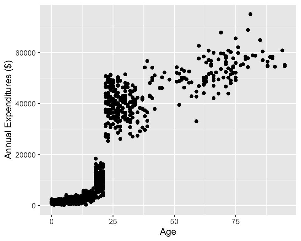

Visualize in more detail: ethnicity, age, and expenditures

dds.discr_Hips_WhnH <- dds.discr %>%  
  filter(ethnicity == "White not Hispanic" | ethnicity == "Hispanic" ) %>% 
  droplevels()   # remove empty factor levels
  

ggplot(data = dds.discr_Hips_WhnH,   
       aes(x = expenditures,
           y = age.cohort)) + 
  geom_boxplot(color="darkgrey") + 
  facet_grid(rows = "ethnicity") +   
  labs(x = "Annual Expenditures ($)",
       y = "Race and ethnicity") +
  geom_jitter(     
    aes(color = ethnicity),      
    alpha = 0.3,      
    show.legend = FALSE,      
    position = position_jitter(     
      height = 0.4))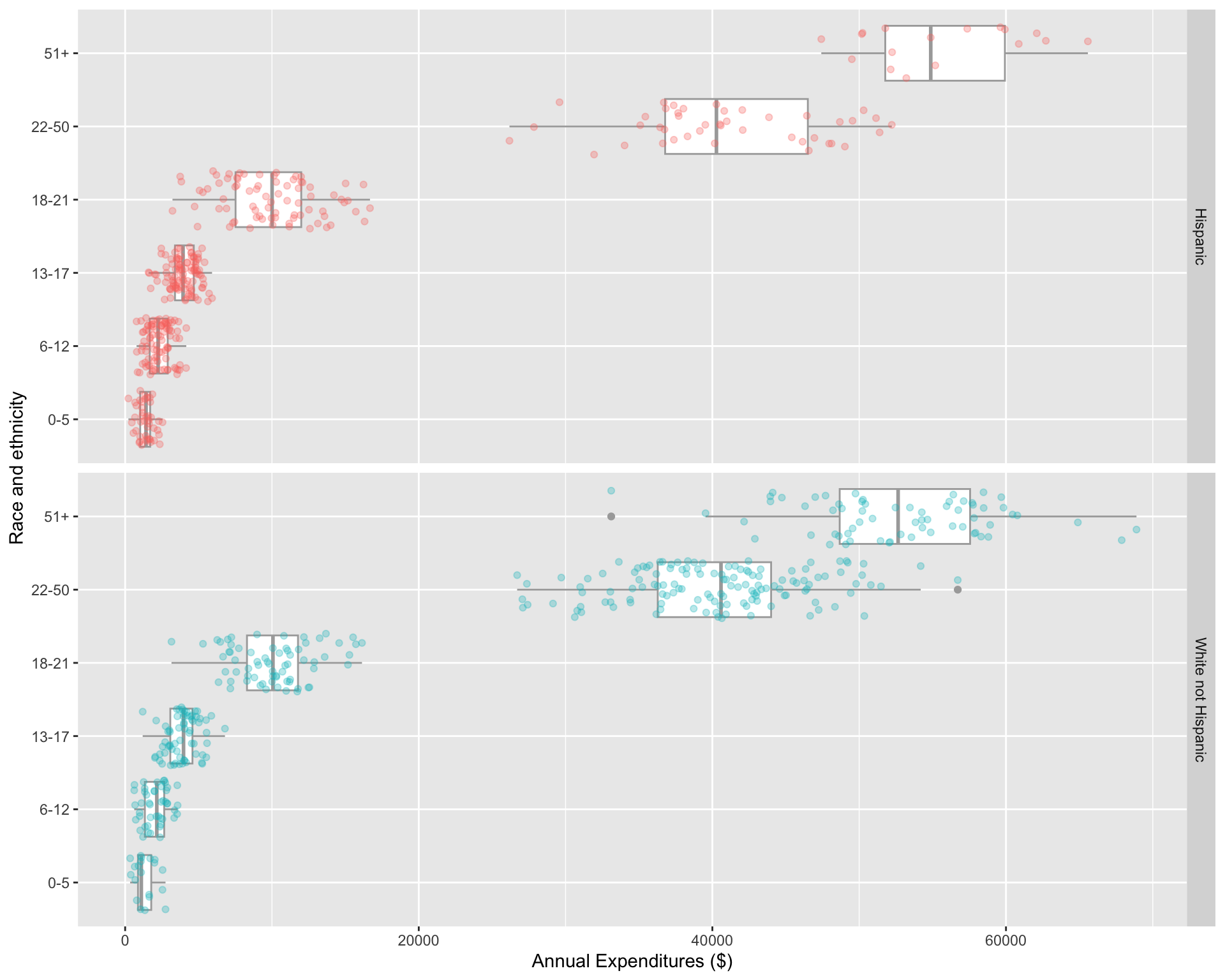

Mean annual DDS expenditures by race/ethnicity

default long format

mean_expend <- dds.discr_Hips_WhnH %>% 
  group_by(ethnicity, age.cohort)%>% 
  summarize(ave = mean(expenditures))

mean_expend

# A tibble: 12 × 3
# Groups:   ethnicity [2]
   ethnicity          age.cohort    ave
   <fct>              <fct>       <dbl>
 1 Hispanic           0-5         1393.
 2 Hispanic           6-12        2312.
 3 Hispanic           13-17       3955.
 4 Hispanic           18-21       9960.
 5 Hispanic           22-50      40924.
 6 Hispanic           51+        55585 
 7 White not Hispanic 0-5         1367.
 8 White not Hispanic 6-12        2052.
 9 White not Hispanic 13-17       3904.
10 White not Hispanic 18-21      10133.
11 White not Hispanic 22-50      40188.
12 White not Hispanic 51+        52670.

wide format

mean_expend_wide <- mean_expend %>% 
  pivot_wider(names_from = ethnicity,
              values_from = ave)

mean_expend_wide

# A tibble: 6 × 3
  age.cohort Hispanic `White not Hispanic`
  <fct>         <dbl>                <dbl>
1 0-5           1393.                1367.
2 6-12          2312.                2052.
3 13-17         3955.                3904.
4 18-21         9960.               10133.
5 22-50        40924.               40188.
6 51+          55585                52670.

Differences in mean annual DDS expenditures by age cohort and race/ethnicity

mean_expend_wide <- mean_expend_wide %>% 
  mutate(diff_mean = `White not Hispanic` - Hispanic)

mean_expend_wide

# A tibble: 6 × 4
  age.cohort Hispanic `White not Hispanic` diff_mean
  <fct>         <dbl>                <dbl>     <dbl>
1 0-5           1393.                1367.     -26.3
2 6-12          2312.                2052.    -260. 
3 13-17         3955.                3904.     -50.9
4 18-21         9960.               10133.     173. 
5 22-50        40924.               40188.    -736. 
6 51+          55585                52670.   -2915.

Question: Are the data sufficient evidence of ethnic discrimination in DDS expenditures when comparing Hispanics with White non-Hispanics?

Summary of data wrangling so far

The pipe %>% to string together commands in sequence
mutate() to add a new variable to a dataset
select() to select columns (or deselect columns with -variable)
filter() to select specific rows
pivot_wider() to reshape a dataset from a long to a wide format

Summarizing data

tabyl() from janitor package to make frequency tables of categorical variables
summarize() to get summary statistics of variables
group_by() to group data by categorical variables before finding summaries