Week 4

mutate(), case_when(), more ggplot2

Published

January 31, 2024

Modified

February 13, 2024

Topics

Learn and apply mutate() to change the data type of a variable
Apply mutate() to calculate a new variable based on other variables in a data.frame.
Apply case_when in a mutate() statement to make a continuous variable categorical
Learn how to mutate() across() multiple columns at once.
Learn to facet and change scales/palettes of ggplots.

Announcements

Class materials for BSTA 526 will be provided in the shared OneDrive folder BSTA_526_W24_class_materials_public.
For today’s class, make sure to download to your computer the folder called part_04, and then open RStudio by double-clicking on the file called part_04.Rproj.
If you have not already done so, please join the BSTA 526 Slack channel and introduce yourself by posting in the #random channel.

Class materials

Readings
One Drive part_04 Project folder

Post-class survey

Please fill out the post-class survey to provide feedback. Thank you!

Homework

See OneDrive folder for homework assignment.
HW 4 due on 2/7.

Recording

In-class recording links are on Sakai. Navigate to Course Materials -> Schedule with links to in-class recordings. Note that the password to the recordings is at the top of the page.

Muddiest points from Week 4

Feedback from post-class surveys

See Week 3 page for Week 3 feedback.

# Load packages
pacman::p_load(tidyverse, 
               readxl, 
               janitor,
               here)

# Load data
smoke_complete <- readxl::read_excel(here("data", "smoke_complete.xlsx"), 
                                     sheet = 1, 
                                     na = "NA")
                                     
# dplyr::glimpse(smoke_complete)

Keyboard shortcut for the pipe (`%>%` or `|>`)

In office hours, someone didn’t know about this fact and wanted to make sure everyone knows about it.

Important keyboard shortcut

In RStudio the keyboard shortcut for the pipe operator %>% (or native pipe |>) is Ctrl + Shift + M (Windows) or Cmd + Shift + M (Mac).

Note: Ctrl + Shift + M also works on a Mac.

The difference between NA value and 0

NA (Not Available)

NA is a special value in R that represents missing or undefined data.
0 is a numeric value representing the number zero. It is a valid and well-defined numerical value in R.
It’s important to handle NA values appropriately in data analysis and to consider their impact on calculations, as operations involving NA may result in NA.

NA + 5  # The result is NA

[1] NA

0 + 5  # The results is 5

[1] 5

x <- c(1, 2, NA, 4)

sum(x)  # The result is NA

[1] NA

# Using the argument na.rm = TRUE, means to ignore the NAs
sum(x, na.rm = TRUE) # The results is 7

[1] 7

x <- c(1, 2, 0, 4)

sum(x) # The result is 7

[1] 7

`across()` and it’s usage

The biggest advantage that across brings is the ability to perform the same data manipulation task to multiple columns.

Below the values in three columns are all set to the mean value using the mean(). I had to write out the function and the variable names three times.

smoke_complete |> 
  mutate(days_to_death = mean(days_to_death, na.rm = TRUE), 
         days_to_birth = mean(days_to_birth, na.rm = TRUE), 
         days_to_last_follow_up = mean(days_to_last_follow_up, na.rm = TRUE)) |> 
  dplyr::glimpse()

Rows: 1,152
Columns: 20
$ primary_diagnosis           <chr> "C34.1", "C34.1", "C34.3", "C34.1", "C34.1…
$ tumor_stage                 <chr> "stage ia", "stage ib", "stage ib", "stage…
$ age_at_diagnosis            <dbl> 24477, 26615, 28171, 27154, 23370, 19025, …
$ vital_status                <chr> "dead", "dead", "dead", "alive", "alive", …
$ morphology                  <chr> "8070/3", "8070/3", "8070/3", "8083/3", "8…
$ days_to_death               <dbl> 852.5637, 852.5637, 852.5637, 852.5637, 85…
$ state                       <chr> "live", "live", "live", "live", "live", "l…
$ tissue_or_organ_of_origin   <chr> "C34.1", "C34.1", "C34.3", "C34.1", "C34.1…
$ days_to_birth               <dbl> -24175.38, -24175.38, -24175.38, -24175.38…
$ site_of_resection_or_biopsy <chr> "C34.1", "C34.1", "C34.3", "C34.1", "C34.1…
$ days_to_last_follow_up      <dbl> 944.8547, 944.8547, 944.8547, 944.8547, 94…
$ cigarettes_per_day          <dbl> 10.9589041, 2.1917808, 1.6438356, 1.095890…
$ years_smoked                <dbl> NA, NA, NA, NA, NA, NA, NA, NA, NA, 26, NA…
$ gender                      <chr> "male", "male", "female", "male", "female"…
$ year_of_birth               <dbl> 1936, 1931, 1927, 1930, 1942, 1953, 1932, …
$ race                        <chr> "white", "asian", "white", "white", "not r…
$ ethnicity                   <chr> "not hispanic or latino", "not hispanic or…
$ year_of_death               <dbl> 2004, 2003, NA, NA, NA, 2005, 2006, NA, NA…
$ bcr_patient_barcode         <chr> "TCGA-18-3406", "TCGA-18-3407", "TCGA-18-3…
$ disease                     <chr> "LUSC", "LUSC", "LUSC", "LUSC", "LUSC", "L…

The same thing is accomplished using across() but we only have to call the mean() function once.

smoke_complete |> 
  mutate(dplyr::across(.cols = c(days_to_death, 
                                 days_to_birth, 
                                 days_to_last_follow_up), 
                       .fns = ~ mean(.x, na.rm = TRUE))) |> 
  dplyr::glimpse()

Rows: 1,152
Columns: 20
$ primary_diagnosis           <chr> "C34.1", "C34.1", "C34.3", "C34.1", "C34.1…
$ tumor_stage                 <chr> "stage ia", "stage ib", "stage ib", "stage…
$ age_at_diagnosis            <dbl> 24477, 26615, 28171, 27154, 23370, 19025, …
$ vital_status                <chr> "dead", "dead", "dead", "alive", "alive", …
$ morphology                  <chr> "8070/3", "8070/3", "8070/3", "8083/3", "8…
$ days_to_death               <dbl> 852.5637, 852.5637, 852.5637, 852.5637, 85…
$ state                       <chr> "live", "live", "live", "live", "live", "l…
$ tissue_or_organ_of_origin   <chr> "C34.1", "C34.1", "C34.3", "C34.1", "C34.1…
$ days_to_birth               <dbl> -24175.38, -24175.38, -24175.38, -24175.38…
$ site_of_resection_or_biopsy <chr> "C34.1", "C34.1", "C34.3", "C34.1", "C34.1…
$ days_to_last_follow_up      <dbl> 944.8547, 944.8547, 944.8547, 944.8547, 94…
$ cigarettes_per_day          <dbl> 10.9589041, 2.1917808, 1.6438356, 1.095890…
$ years_smoked                <dbl> NA, NA, NA, NA, NA, NA, NA, NA, NA, 26, NA…
$ gender                      <chr> "male", "male", "female", "male", "female"…
$ year_of_birth               <dbl> 1936, 1931, 1927, 1930, 1942, 1953, 1932, …
$ race                        <chr> "white", "asian", "white", "white", "not r…
$ ethnicity                   <chr> "not hispanic or latino", "not hispanic or…
$ year_of_death               <dbl> 2004, 2003, NA, NA, NA, 2005, 2006, NA, NA…
$ bcr_patient_barcode         <chr> "TCGA-18-3406", "TCGA-18-3407", "TCGA-18-3…
$ disease                     <chr> "LUSC", "LUSC", "LUSC", "LUSC", "LUSC", "L…

Links to check out

`~` and `.x`

We’ve seen the ~ and .x used with dplyr::across(). We will see them again later when we get to the package purrr.

In the tidyverse, ~ and .x are used to create what they call lambda functions which are part of the purrr syntax. We have not talked about functions yet, but purrr package and the dplyr::across() function allow you to specify functions to apply in a few different ways:

A named function, e.g. mean.

smoke_complete |> 
  mutate(dplyr::across(.cols = c(days_to_death, 
                                 days_to_birth, 
                                 days_to_last_follow_up), 
                       .fns = mean)) |> 
  dplyr::glimpse()

Rows: 1,152
Columns: 20
$ primary_diagnosis           <chr> "C34.1", "C34.1", "C34.3", "C34.1", "C34.1…
$ tumor_stage                 <chr> "stage ia", "stage ib", "stage ib", "stage…
$ age_at_diagnosis            <dbl> 24477, 26615, 28171, 27154, 23370, 19025, …
$ vital_status                <chr> "dead", "dead", "dead", "alive", "alive", …
$ morphology                  <chr> "8070/3", "8070/3", "8070/3", "8083/3", "8…
$ days_to_death               <dbl> NA, NA, NA, NA, NA, NA, NA, NA, NA, NA, NA…
$ state                       <chr> "live", "live", "live", "live", "live", "l…
$ tissue_or_organ_of_origin   <chr> "C34.1", "C34.1", "C34.3", "C34.1", "C34.1…
$ days_to_birth               <dbl> -24175.38, -24175.38, -24175.38, -24175.38…
$ site_of_resection_or_biopsy <chr> "C34.1", "C34.1", "C34.3", "C34.1", "C34.1…
$ days_to_last_follow_up      <dbl> NA, NA, NA, NA, NA, NA, NA, NA, NA, NA, NA…
$ cigarettes_per_day          <dbl> 10.9589041, 2.1917808, 1.6438356, 1.095890…
$ years_smoked                <dbl> NA, NA, NA, NA, NA, NA, NA, NA, NA, 26, NA…
$ gender                      <chr> "male", "male", "female", "male", "female"…
$ year_of_birth               <dbl> 1936, 1931, 1927, 1930, 1942, 1953, 1932, …
$ race                        <chr> "white", "asian", "white", "white", "not r…
$ ethnicity                   <chr> "not hispanic or latino", "not hispanic or…
$ year_of_death               <dbl> 2004, 2003, NA, NA, NA, 2005, 2006, NA, NA…
$ bcr_patient_barcode         <chr> "TCGA-18-3406", "TCGA-18-3407", "TCGA-18-3…
$ disease                     <chr> "LUSC", "LUSC", "LUSC", "LUSC", "LUSC", "L…

Note

Above, just using the function name, we are not able to provide the additional argument na.rm = TRUE to the mean() function, so the columns are now all NA values because there were missing (NA) values in those columns.

An anonymous function, e.g. \(x) x + 1 or function(x) x + 1.

This has not been covered yet. R lets you specify your own functions and there are two basic ways to do it.

smoke_complete |> 
  mutate(dplyr::across(.cols = c(days_to_death, 
                                 days_to_birth, 
                                 days_to_last_follow_up), 
                       .fns = \(x) mean(x, na.rm = TRUE))) |> 
  dplyr::glimpse()

Rows: 1,152
Columns: 20
$ primary_diagnosis           <chr> "C34.1", "C34.1", "C34.3", "C34.1", "C34.1…
$ tumor_stage                 <chr> "stage ia", "stage ib", "stage ib", "stage…
$ age_at_diagnosis            <dbl> 24477, 26615, 28171, 27154, 23370, 19025, …
$ vital_status                <chr> "dead", "dead", "dead", "alive", "alive", …
$ morphology                  <chr> "8070/3", "8070/3", "8070/3", "8083/3", "8…
$ days_to_death               <dbl> 852.5637, 852.5637, 852.5637, 852.5637, 85…
$ state                       <chr> "live", "live", "live", "live", "live", "l…
$ tissue_or_organ_of_origin   <chr> "C34.1", "C34.1", "C34.3", "C34.1", "C34.1…
$ days_to_birth               <dbl> -24175.38, -24175.38, -24175.38, -24175.38…
$ site_of_resection_or_biopsy <chr> "C34.1", "C34.1", "C34.3", "C34.1", "C34.1…
$ days_to_last_follow_up      <dbl> 944.8547, 944.8547, 944.8547, 944.8547, 94…
$ cigarettes_per_day          <dbl> 10.9589041, 2.1917808, 1.6438356, 1.095890…
$ years_smoked                <dbl> NA, NA, NA, NA, NA, NA, NA, NA, NA, 26, NA…
$ gender                      <chr> "male", "male", "female", "male", "female"…
$ year_of_birth               <dbl> 1936, 1931, 1927, 1930, 1942, 1953, 1932, …
$ race                        <chr> "white", "asian", "white", "white", "not r…
$ ethnicity                   <chr> "not hispanic or latino", "not hispanic or…
$ year_of_death               <dbl> 2004, 2003, NA, NA, NA, 2005, 2006, NA, NA…
$ bcr_patient_barcode         <chr> "TCGA-18-3406", "TCGA-18-3407", "TCGA-18-3…
$ disease                     <chr> "LUSC", "LUSC", "LUSC", "LUSC", "LUSC", "L…

smoke_complete |> 
  mutate(dplyr::across(.cols = c(days_to_death, 
                                 days_to_birth, 
                                 days_to_last_follow_up), 
                       .fns = function(x) mean(x, na.rm = TRUE))) |> 
  dplyr::glimpse()

Rows: 1,152
Columns: 20
$ primary_diagnosis           <chr> "C34.1", "C34.1", "C34.3", "C34.1", "C34.1…
$ tumor_stage                 <chr> "stage ia", "stage ib", "stage ib", "stage…
$ age_at_diagnosis            <dbl> 24477, 26615, 28171, 27154, 23370, 19025, …
$ vital_status                <chr> "dead", "dead", "dead", "alive", "alive", …
$ morphology                  <chr> "8070/3", "8070/3", "8070/3", "8083/3", "8…
$ days_to_death               <dbl> 852.5637, 852.5637, 852.5637, 852.5637, 85…
$ state                       <chr> "live", "live", "live", "live", "live", "l…
$ tissue_or_organ_of_origin   <chr> "C34.1", "C34.1", "C34.3", "C34.1", "C34.1…
$ days_to_birth               <dbl> -24175.38, -24175.38, -24175.38, -24175.38…
$ site_of_resection_or_biopsy <chr> "C34.1", "C34.1", "C34.3", "C34.1", "C34.1…
$ days_to_last_follow_up      <dbl> 944.8547, 944.8547, 944.8547, 944.8547, 94…
$ cigarettes_per_day          <dbl> 10.9589041, 2.1917808, 1.6438356, 1.095890…
$ years_smoked                <dbl> NA, NA, NA, NA, NA, NA, NA, NA, NA, 26, NA…
$ gender                      <chr> "male", "male", "female", "male", "female"…
$ year_of_birth               <dbl> 1936, 1931, 1927, 1930, 1942, 1953, 1932, …
$ race                        <chr> "white", "asian", "white", "white", "not r…
$ ethnicity                   <chr> "not hispanic or latino", "not hispanic or…
$ year_of_death               <dbl> 2004, 2003, NA, NA, NA, 2005, 2006, NA, NA…
$ bcr_patient_barcode         <chr> "TCGA-18-3406", "TCGA-18-3407", "TCGA-18-3…
$ disease                     <chr> "LUSC", "LUSC", "LUSC", "LUSC", "LUSC", "L…

Note

Now we are able to use the additional argument na.rm = TRUE and the columns are now the means of the valid values in those columns.

A purrr-style lambda function, e.g. ~ mean(.x, na.rm = TRUE)

We use ~ to indicate that we are supplying a lambda function and we use .x as a placeholder for the argument within our lambda function to indicate where to use the variable.

smoke_complete |> 
  mutate(dplyr::across(.cols = c(days_to_death, 
                                 days_to_birth, 
                                 days_to_last_follow_up), 
                       .fns = ~ mean(.x, na.rm = TRUE))) |> 
  dplyr::glimpse()

Rows: 1,152
Columns: 20
$ primary_diagnosis           <chr> "C34.1", "C34.1", "C34.3", "C34.1", "C34.1…
$ tumor_stage                 <chr> "stage ia", "stage ib", "stage ib", "stage…
$ age_at_diagnosis            <dbl> 24477, 26615, 28171, 27154, 23370, 19025, …
$ vital_status                <chr> "dead", "dead", "dead", "alive", "alive", …
$ morphology                  <chr> "8070/3", "8070/3", "8070/3", "8083/3", "8…
$ days_to_death               <dbl> 852.5637, 852.5637, 852.5637, 852.5637, 85…
$ state                       <chr> "live", "live", "live", "live", "live", "l…
$ tissue_or_organ_of_origin   <chr> "C34.1", "C34.1", "C34.3", "C34.1", "C34.1…
$ days_to_birth               <dbl> -24175.38, -24175.38, -24175.38, -24175.38…
$ site_of_resection_or_biopsy <chr> "C34.1", "C34.1", "C34.3", "C34.1", "C34.1…
$ days_to_last_follow_up      <dbl> 944.8547, 944.8547, 944.8547, 944.8547, 94…
$ cigarettes_per_day          <dbl> 10.9589041, 2.1917808, 1.6438356, 1.095890…
$ years_smoked                <dbl> NA, NA, NA, NA, NA, NA, NA, NA, NA, 26, NA…
$ gender                      <chr> "male", "male", "female", "male", "female"…
$ year_of_birth               <dbl> 1936, 1931, 1927, 1930, 1942, 1953, 1932, …
$ race                        <chr> "white", "asian", "white", "white", "not r…
$ ethnicity                   <chr> "not hispanic or latino", "not hispanic or…
$ year_of_death               <dbl> 2004, 2003, NA, NA, NA, 2005, 2006, NA, NA…
$ bcr_patient_barcode         <chr> "TCGA-18-3406", "TCGA-18-3407", "TCGA-18-3…
$ disease                     <chr> "LUSC", "LUSC", "LUSC", "LUSC", "LUSC", "L…

Links to check out

Some of these are purrr focused which we have not covered yet. Others use dplyr::across() withing the dplyr::summarize() function which we will be covering soon

Exceptions where we have seen the `~` used

In class, we have seen three instances where the ~ is used that is not for a lambda function.

`case_when`

smoke_complete |> 
  mutate(cigarettes_category = case_when(
      cigarettes_per_day < 6 ~ "0-5", 
      cigarettes_per_day >= 6 ~ "6+"
    )) |> 
  mutate(cigarettes_category = factor(cigarettes_category)) |> 
  janitor::tabyl(cigarettes_category)

 cigarettes_category    n    percent
                 0-5 1100 0.95486111
                  6+   52 0.04513889

`facet_wrap`

ggplot(data = smoke_complete, 
       aes(x = age_at_diagnosis, 
           y = cigarettes_per_day)) + 
  geom_point() + 
  facet_wrap(~ disease)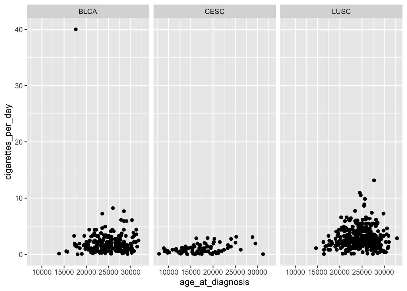

Per the facet_wrap vignettte:

For compatibility with the classic interface, can also be a formula or character vector. Use either a one sided formula, ~a + b, or a character vector, c("a", "b").

Here it is being used to specify a formula.

Though per the vignette, the vars() function is preferred syntax:

ggplot(data = smoke_complete, 
       aes(x = age_at_diagnosis, 
           y = cigarettes_per_day)) + 
  geom_point() + 
  facet_wrap(ggplot2::vars(disease))

`facet_grid`

ggplot(data = smoke_complete, 
       aes(x = age_at_diagnosis, 
           y = cigarettes_per_day)) + 
  geom_point() + 
  facet_grid(disease ~ vital_status)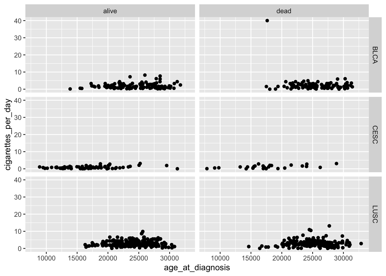

Per the facet_grid vignettte:

For compatibility with the classic interface, rows can also be a formula with the rows (of the tabular display) on the LHS and the columns (of the tabular display) on the RHS; the dot in the formula is used to indicate there should be no faceting on this dimension (either row or column).

Again, it is being used to specify a formula.

Though per the vignette, the ggplot2::vars() function with the arguments rows and cols seems to be preferred:

ggplot(data = smoke_complete, 
       aes(x = age_at_diagnosis, 
           y = cigarettes_per_day)) + 
  geom_point() + 
  facet_grid(rows = ggplot2::vars(disease), 
             cols = ggplot2::vars(vital_status))

Note: dplyr::vars() and dplyr::ggplot2() are the same function in different packages and can be used interchangeably.

`case_when` vs. `if_else`

In dplyr, both if_else() and case_when() are used for conditional transformations, but they have different use cases and behaviors.

if_else function

if_else() is designed for simple vectorized conditions and is particularly useful when you have a binary condition (i.e., two possible outcomes).
It evaluates a condition for each element of a vector and returns one of two values based on whether the condition is TRUE or FALSE.

smoke_complete |> 
  mutate(cigarettes_category = dplyr::if_else(cigarettes_per_day < 6, "0-5", "6+")) |> 
  mutate(cigarettes_category = factor(cigarettes_category)) |> 
  janitor::tabyl(cigarettes_category)

 cigarettes_category    n    percent
                 0-5 1100 0.95486111
                  6+   52 0.04513889

In this example, the column cigarettes_category is assigned the value “0-5” if cigarettes_per_day is less than 6 and “6+” otherwise.

case_when() function

case_when() is more versatile and is suitable for handling multiple conditions with multiple possible outcomes. It is essentially a vectorized form of a switch or if_else chain.
It allows you to specify multiple conditions and their corresponding values.

smoke_complete |> 
  mutate(cigarettes_category = case_when(
      cigarettes_per_day < 2 ~ "0 to 2", 
      cigarettes_per_day < 4 ~ "2 to 4", 
      cigarettes_per_day < 6 ~ "4 to 6", 
      cigarettes_per_day >= 6 ~ "6+"
    )) |> 
  mutate(cigarettes_category = factor(cigarettes_category)) |> 
  janitor::tabyl(cigarettes_category)

 cigarettes_category   n    percent
              0 to 2 455 0.39496528
              2 to 4 493 0.42795139
              4 to 6 152 0.13194444
                  6+  52 0.04513889

In this example, the column cigarettes_category is assigned the value “0 to 2” if cigarettes_per_day is less than 2, “2 to 4” if less than 4 (but greater than 2), “4 to 6” if less than 6 (but greater than 4), and “6+” otherwise.

Use if_else() when you have a simple binary condition, and use case_when() when you need to handle multiple conditions with different outcomes. case_when() is more flexible and expressive when dealing with complex conditional transformations.

The difference between a theme and and a palette.

In ggplot2, a theme and a palette serve different purposes and are used in different contexts. In summary, a theme controls the overall appearance of the plot, while a palette is specifically related to the colors used to represent different groups or levels within the data. Both themes and palettes contribute to visual appeal and readability of your plot.

Theme:

A theme in ggplot2 refers to the overall visual appearance of the plot. It includes elements such as fonts, colors, grid lines, background, and other visual attributes that define the look and feel of the entire plot.
Themes are set using functions like theme_minimal(), theme_classic(), or custom themes created with the theme() function. Themes control the global appearance of the plot.

library(ggplot2)

# Example using theme_minimal()
ggplot(data = smoke_complete, 
       aes(x = age_at_diagnosis, 
           y = cigarettes_per_day)) + 
  geom_point() + 
  theme_minimal()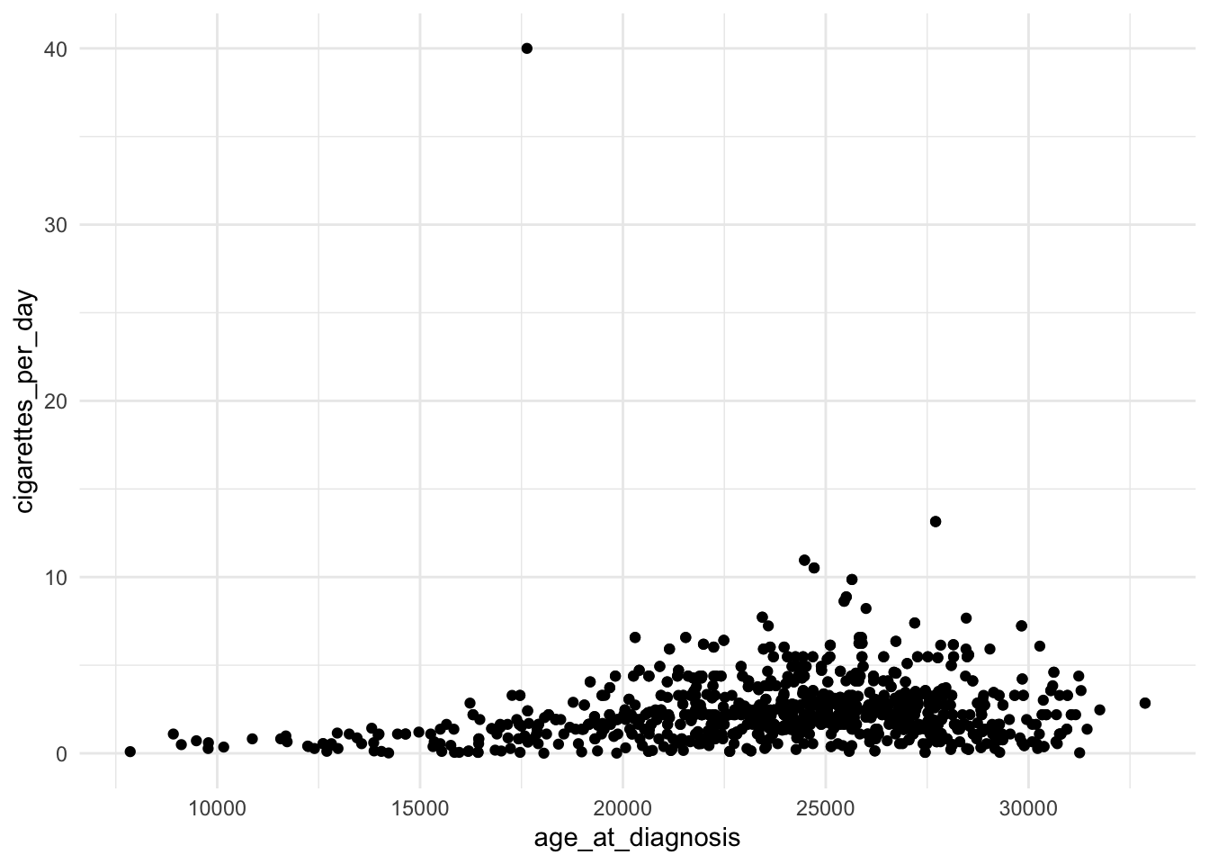

Palette:

A palette, on the other hand, refers to a set of colors used to represent different levels or categories in the data. It is particularly relevant when working with categorical or discrete data where you want to distinguish between different groups.
Palettes are set using functions like scale_fill_manual() or scale_color_manual(). You can specify a vector of colors or use pre-defined palettes from packages like RColorBrewer or viridis (we looked at the viridis package in class).

# Example using a color palette
ggplot(data = smoke_complete, 
       aes(x = age_at_diagnosis, 
           y = cigarettes_per_day, 
           color = disease)) + 
  geom_point() +
  scale_color_manual(values = c("red", 
                                "blue", 
                                "green"))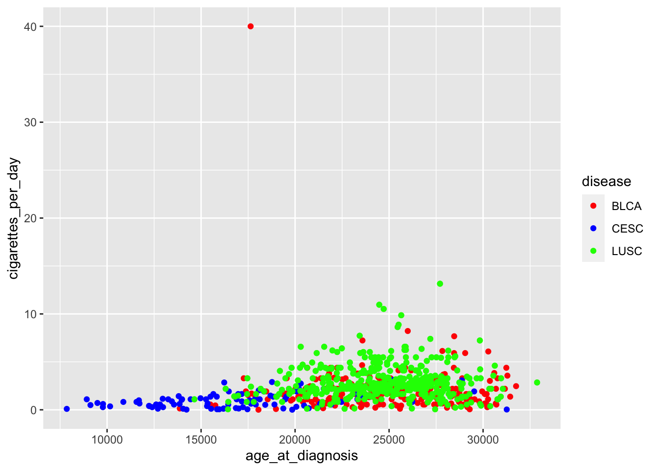

Be careful what you pipe to and from

An error came up where a data frame was being piped to a function that did not accept a data frame as an argument (it accepted a vector)

# starwars data frame was loaded earlier with the ggplot2 package

starwars |>  
  dplyr::n_distinct(species)

Error in list2(...): object 'species' not found

starwars is a data frame.
dplyr::n_distinct() only accepts a vector as an argument (check the help ?dplyr::n_distinct)

So we need to pipe a vector to the dplyr::n_distinct() function:

starwars |> 
  dplyr::select(species) |> 
  dplyr::n_distinct()

[1] 38

dplyr::select() accepts a data frame as its first argument and it return a vector (see the help ?dplyr::select) which we can then pipe to dplyr::n_distinct().

The %>% or |> takes the output of the expression on its left and passes it as the first argument to the function on its right. The class / type of output on the left needs to agree or be acceptable as the first argument to the function on the right.

Other muddy points

Remembering applicable functions. Troubleshooting.

This gets better with experience. You are all still very new to R so be patient with yourself.

How to organize all of the material to understand the structure of how the R language works, rather than to keep track of all of the commands in an anecdotal way.

Again, I think that this gets better with experience. Though the R language, being open source, a lot of syntax is package dependent. So you need to be careful that some of the syntax we use with dplyr and the tidyverse will be different in base R or in other packages. This is something that comes with open source software (compared to Stata or SAS). The good news is that learning to use packages sets you up to better learn newer (to you) packages down the road.

Topics

Announcements

Class materials

Post-class survey

Homework

Recording

Muddiest points from Week 4

Keyboard shortcut for the pipe (%>% or |>)

The difference between NA value and 0

NA (Not Available)

across() and it’s usage

Links to check out

~ and .x

Links to check out

Exceptions where we have seen the ~ used

case_when

facet_wrap

facet_grid

case_when vs. if_else

The difference between a theme and and a palette.

Be careful what you pipe to and from

Other muddy points

Keyboard shortcut for the pipe (`%>%` or `|>`)

`across()` and it’s usage

`~` and `.x`

Exceptions where we have seen the `~` used

`case_when`

`facet_wrap`

`facet_grid`

`case_when` vs. `if_else`