9: Iteration

BSTA 526: R Programming for Health Data Science

Meike Niederhausen, PhD & Jessica Minnier, PhD

OHSU-PSU School of Public Health

2026-03-05

1 Welcome to R Programming: Part 9!

Today we will learn about iterating in R.


Before you get started:

Remember to save this notebook under a new name, such as part_09_b526_YOURNAME.qmd.


  • Load the packages in the setup code chunk

1.1 Learning Objectives

  • Introduce statistical modeling and learn how to fit a simple linear regression model and run a t-test in R
  • Learn how to use broom functions to tidy up statistical model output
  • Learn about for loops
  • Understand how to apply a function to a list
  • Learn how to iterate over a list using map() functions from the purrr package

2 Brief Introduction to Statistics in R

  • A brief introduction on statistical models in R and how to extract output in a “tidy” way
  • We will be using statistical models as iteration examples and applying purrr::map()

2.1 This is just a brief modeling overview!

  • This is not meant to be a comprehensive course in statistics!!
  • Just showing some basic techniques.
  • If you want to learn more about statistical modeling, here are some resources:

If you’ve worked with statistical models and tests in R, you know they have an…eclectic way of inputting data and outputting results. The inputs and outputs are not standardized or consistent.

2.2 Linear Regression

  • A linear regression model uses least squares estimation to fit the closest linear line to the model (very simplistic explanation).
  • The linear regression formula is often written as:

\[Y = \beta_0 + \beta_1 \cdot X + error\]

  • \(Y\) is a numeric continuous measurement (the “outcome” or “dependent variable”)
  • \(X\) is a covariate (or “predictor” or “independent variable”).
    • \(X\) can be numeric or categorical (in R, this can be numeric, factor, character, or boolean).
  • \(\beta_0\) denotes the intercept of the line
  • \(\beta_1\) denotes the slope of the line, or our coefficient.
  • The error is assumed to normally distributed (Gaussian) with mean 0.

2.3 R formula for linear regression

  • In R, this translates to using a formula argument in the lm() function of the format outcome ~ predictor (the intercept is implied):

Y ~ X

Or if we have multiple predictors/covariates (independent variables), perhaps:

Y ~ A + B + C

  • The function lm() is in the stats package, which is automatically loaded with every R session.
    • So you don’t need to call library(stats) or p_load(stats) to use it.
  • Use the Palmer penguins data set
  • Outcome: body_mass_g (continuous)
  • Independent variables: species and sex

outcome ~ independent variables
body_mass_g ~ species + sex

  • Categorical independent variables
    • R converts categorical predictors, such as species and sex, into categories in the model
    • The estimates are interpreted as the expected mean differences in body mass compared to the reference group.
    • The reference group is by default the first alphabetical category.
      • If you wish to change the reference group, you need to use factors.
  • If you have not taken BSTA 512/612, or a similar linear regression class, you can learn more about linear regression section in Learning Statistics with R!.

Always read the documentation! ?lm

fit_lm <- lm(
  # formula: Y/dependent variable/outcome on left 
  # ~ X's independent variables on right
  body_mass_g ~ species + sex,
  data = penguins
)
  • This prints out the formula and the coefficient estimates, nothing else
fit_lm

Call:
lm(formula = body_mass_g ~ species + sex, data = penguins)

Coefficients:
     (Intercept)  speciesChinstrap     speciesGentoo           sexmale  
         3372.39             26.92           1377.86            667.56  
  • This prints out the coefficient estimates as well as statistics and p-values
summary(fit_lm)

Call:
lm(formula = body_mass_g ~ species + sex, data = penguins)

Residuals:
    Min      1Q  Median      3Q     Max 
-816.87 -217.80  -16.87  227.61  882.20 

Coefficients:
                 Estimate Std. Error t value Pr(>|t|)    
(Intercept)       3372.39      31.43 107.308   <2e-16 ***
speciesChinstrap    26.92      46.48   0.579    0.563    
speciesGentoo     1377.86      39.10  35.236   <2e-16 ***
sexmale            667.56      34.70  19.236   <2e-16 ***
---
Signif. codes:  0 '***' 0.001 '**' 0.01 '*' 0.05 '.' 0.1 ' ' 1

Residual standard error: 316.6 on 329 degrees of freedom
  (11 observations deleted due to missingness)
Multiple R-squared:  0.8468,    Adjusted R-squared:  0.8454 
F-statistic: 606.1 on 3 and 329 DF,  p-value: < 2.2e-16
  • What kind of object is fit_lm?
class(fit_lm)
[1] "lm"
  • Look at diagnostic plots
# plot(fit_lm)
  • What’s in fit_lm?
str(fit_lm)
List of 14
 $ coefficients : Named num [1:4] 3372.4 26.9 1377.9 667.6
  ..- attr(*, "names")= chr [1:4] "(Intercept)" "speciesChinstrap" "speciesGentoo" "sexmale"
 $ residuals    : Named num [1:333] -289.9 427.6 -122.4 77.6 -389.9 ...
  ..- attr(*, "names")= chr [1:333] "1" "2" "3" "5" ...
 $ effects      : Named num [1:333] -76772 -4381 11225 6090 -376 ...
  ..- attr(*, "names")= chr [1:333] "(Intercept)" "speciesChinstrap" "speciesGentoo" "sexmale" ...
 $ rank         : int 4
 $ fitted.values: Named num [1:333] 4040 3372 3372 3372 4040 ...
  ..- attr(*, "names")= chr [1:333] "1" "2" "3" "5" ...
 $ assign       : int [1:4] 0 1 1 2
 $ qr           :List of 5
  ..$ qr   : num [1:333, 1:4] -18.2483 0.0548 0.0548 0.0548 0.0548 ...
  .. ..- attr(*, "dimnames")=List of 2
  .. .. ..$ : chr [1:333] "1" "2" "3" "5" ...
  .. .. ..$ : chr [1:4] "(Intercept)" "speciesChinstrap" "speciesGentoo" "sexmale"
  .. ..- attr(*, "assign")= int [1:4] 0 1 1 2
  .. ..- attr(*, "contrasts")=List of 2
  .. .. ..$ species: chr "contr.treatment"
  .. .. ..$ sex    : chr "contr.treatment"
  ..$ qraux: num [1:4] 1.05 1.03 1.05 1.05
  ..$ pivot: int [1:4] 1 2 3 4
  ..$ tol  : num 1e-07
  ..$ rank : int 4
  ..- attr(*, "class")= chr "qr"
 $ df.residual  : int 329
 $ na.action    : 'omit' Named int [1:11] 4 9 10 11 12 48 179 219 257 269 ...
  ..- attr(*, "names")= chr [1:11] "4" "9" "10" "11" ...
 $ contrasts    :List of 2
  ..$ species: chr "contr.treatment"
  ..$ sex    : chr "contr.treatment"
 $ xlevels      :List of 2
  ..$ species: chr [1:3] "Adelie" "Chinstrap" "Gentoo"
  ..$ sex    : chr [1:2] "female" "male"
 $ call         : language lm(formula = body_mass_g ~ species + sex, data = penguins)
 $ terms        :Classes 'terms', 'formula'  language body_mass_g ~ species + sex
  .. ..- attr(*, "variables")= language list(body_mass_g, species, sex)
  .. ..- attr(*, "factors")= int [1:3, 1:2] 0 1 0 0 0 1
  .. .. ..- attr(*, "dimnames")=List of 2
  .. .. .. ..$ : chr [1:3] "body_mass_g" "species" "sex"
  .. .. .. ..$ : chr [1:2] "species" "sex"
  .. ..- attr(*, "term.labels")= chr [1:2] "species" "sex"
  .. ..- attr(*, "order")= int [1:2] 1 1
  .. ..- attr(*, "intercept")= int 1
  .. ..- attr(*, "response")= int 1
  .. ..- attr(*, ".Environment")=<environment: R_GlobalEnv> 
  .. ..- attr(*, "predvars")= language list(body_mass_g, species, sex)
  .. ..- attr(*, "dataClasses")= Named chr [1:3] "numeric" "factor" "factor"
  .. .. ..- attr(*, "names")= chr [1:3] "body_mass_g" "species" "sex"
 $ model        :'data.frame':  333 obs. of  3 variables:
  ..$ body_mass_g: int [1:333] 3750 3800 3250 3450 3650 3625 4675 3200 3800 4400 ...
  ..$ species    : Factor w/ 3 levels "Adelie","Chinstrap",..: 1 1 1 1 1 1 1 1 1 1 ...
  ..$ sex        : Factor w/ 2 levels "female","male": 2 1 1 1 2 1 2 1 2 2 ...
  ..- attr(*, "terms")=Classes 'terms', 'formula'  language body_mass_g ~ species + sex
  .. .. ..- attr(*, "variables")= language list(body_mass_g, species, sex)
  .. .. ..- attr(*, "factors")= int [1:3, 1:2] 0 1 0 0 0 1
  .. .. .. ..- attr(*, "dimnames")=List of 2
  .. .. .. .. ..$ : chr [1:3] "body_mass_g" "species" "sex"
  .. .. .. .. ..$ : chr [1:2] "species" "sex"
  .. .. ..- attr(*, "term.labels")= chr [1:2] "species" "sex"
  .. .. ..- attr(*, "order")= int [1:2] 1 1
  .. .. ..- attr(*, "intercept")= int 1
  .. .. ..- attr(*, "response")= int 1
  .. .. ..- attr(*, ".Environment")=<environment: R_GlobalEnv> 
  .. .. ..- attr(*, "predvars")= language list(body_mass_g, species, sex)
  .. .. ..- attr(*, "dataClasses")= Named chr [1:3] "numeric" "factor" "factor"
  .. .. .. ..- attr(*, "names")= chr [1:3] "body_mass_g" "species" "sex"
  ..- attr(*, "na.action")= 'omit' Named int [1:11] 4 9 10 11 12 48 179 219 257 269 ...
  .. ..- attr(*, "names")= chr [1:11] "4" "9" "10" "11" ...
 - attr(*, "class")= chr "lm"
  • Extract coefficients from a list
    • Remember [["coefficients]] is equivalent to $coefficients here.
fit_lm$coefficients
     (Intercept) speciesChinstrap    speciesGentoo          sexmale 
      3372.38681         26.92385       1377.85803        667.55515 
  • Can use pluck to go deeper in the index
fit_lm %>% pluck(coefficients, "sexmale")
[1] 667.5552

2.4 Table of model estimates and p-values

  • Goal: Create a table with model estimates and p-values
    • Add confidence intervals?
  • coef(summary(fit_lm)) and confint(fit_lm)) can be used
    • … but they are a bit of work and
    • not standardized across all the statistical methods/models
    • (also, confusing, why do we need to use coef on the summary and confint on the original model? Who knows…)
coef(summary(fit_lm))
                   Estimate Std. Error     t value      Pr(>|t|)
(Intercept)      3372.38681   31.42724 107.3077587 4.341117e-258
speciesChinstrap   26.92385   46.48341   0.5792142  5.628410e-01
speciesGentoo    1377.85803   39.10409  35.2356475 1.051670e-113
sexmale           667.55515   34.70397  19.2356975  8.729411e-56
confint(fit_lm)
                      2.5 %    97.5 %
(Intercept)      3310.56312 3434.2105
speciesChinstrap  -64.51835  118.3661
speciesGentoo    1300.93243 1454.7836
sexmale           599.28547  735.8248

Enter broom!

2.5 broom for tidy()-ing statistical output

  • The broom package is truly a life changing package for statisticians.
  • 3 main functions in broom:
    • tidy() - most of the output you want, including coefficients and p-values
    • glance() - additional model measures, including R-squared, log likelihood, and AIC/BIC
    • augment() - make predictions with your model using new data
  • We will mostly use tidy() and glance() for right now.
  • Argument: a (regression) model object
    • many types of models or even simple tests work, such as t-test, etc.
  • Output: a cleaned up tibble of model results
tidy(fit_lm)
# A tibble: 4 × 5
  term             estimate std.error statistic   p.value
  <chr>               <dbl>     <dbl>     <dbl>     <dbl>
1 (Intercept)        3372.       31.4   107.    4.34e-258
2 speciesChinstrap     26.9      46.5     0.579 5.63e-  1
3 speciesGentoo      1378.       39.1    35.2   1.05e-113
4 sexmale             668.       34.7    19.2   8.73e- 56
  • We can ask for confidence intervals:
tidy(fit_lm, conf.int = TRUE)
# A tibble: 4 × 7
  term             estimate std.error statistic   p.value conf.low conf.high
  <chr>               <dbl>     <dbl>     <dbl>     <dbl>    <dbl>     <dbl>
1 (Intercept)        3372.       31.4   107.    4.34e-258   3311.      3434.
2 speciesChinstrap     26.9      46.5     0.579 5.63e-  1    -64.5      118.
3 speciesGentoo      1378.       39.1    35.2   1.05e-113   1301.      1455.
4 sexmale             668.       34.7    19.2   8.73e- 56    599.       736.
  • We can save this tibble and make it prettier with tidyverse functions and gt:
# save the tidy output
lm_tidy_output <- tidy(fit_lm, conf.int = TRUE)

Format p-value nicely with scales::label_pvalue():

# an example of using scales::label_pvalue to format p-value nicely
scales::label_pvalue(accuracy = 0.001)(0.2354464)
[1] "0.235"
scales::label_pvalue(accuracy = 0.001)(0.00023)
[1] "<0.001"
# apply to lm output:
lm_tidy_output %>% 
  select(term, estimate, conf.low, conf.high, p.value) %>%
  mutate(
    # use the scales package to format the p-value nicely
    p.value = scales::label_pvalue(accuracy = 0.001)(p.value),
    # round numeric columns to 1 digit
    across(.cols = where(is.numeric),
           .fns = ~round(.x, digits = 1))
    ) %>%
  # use gt to make nice html table
  gt()
term estimate conf.low conf.high p.value
(Intercept) 3372.4 3310.6 3434.2 <0.001
speciesChinstrap 26.9 -64.5 118.4 0.563
speciesGentoo 1377.9 1300.9 1454.8 <0.001
sexmale 667.6 599.3 735.8 <0.001
  • Use broom::glance() to obtain model fit estimates, statistics, and tests.
glance(fit_lm) %>% gt()
r.squared adj.r.squared sigma statistic p.value df logLik AIC BIC deviance df.residual nobs
0.8467935 0.8453965 316.6081 606.1427 1.269875e-133 3 -2387.797 4785.594 4804.634 32979185 329 333

2.6 gtsummary package for statistical tables

  • The gtsummary package has several useful functions for creating nicely summarized output.
  • Here’s the regression table:
tbl_regression(fit_lm)
Characteristic Beta 95% CI1 p-value
species


    Adelie
    Chinstrap 27 -65, 118 0.6
    Gentoo 1,378 1,301, 1,455 <0.001
sex


    female
    male 668 599, 736 <0.001
1 CI = Confidence Interval
  • If you prefer the global p-value for a multi-category covariate such as species:
tbl_regression(fit_lm) %>%
  add_global_p(keep = TRUE)
Characteristic Beta 95% CI1 p-value
species

<0.001
    Adelie
    Chinstrap 27 -65, 118 0.6
    Gentoo 1,378 1,301, 1,455 <0.001
sex

<0.001
    female
    male 668 599, 736 <0.001
1 CI = Confidence Interval
  • There are many ways to use and customize these tables
    • that we will talk about in part 10.

2.7 t-test (independent samples)

  • Briefly, a (independent samples) t-test is used to test whether the means between two groups are different.
    • The measurements must be numeric.
    • The null hypothesis for a t-test is that the two means are equal, and the alternative hypothesis is that they are not equal.
    • See Day 11 materials from BSTA 511 for more information.
  • The t-test formula in R is similar to a linear regression
    • the continuous numerical measurement is on the left side of the ~ and
    • on the right side is the grouping variable.
  • Look at the ?t.test documentation
    • to determine whether this is a two-sided t-test, and
    • whether it assumes the variances in each group are equal.
    • How would you perform a paired t-test?
t.test(body_mass_g ~ sex, data = penguins)

    Welch Two Sample t-test

data:  body_mass_g by sex
t = -8.5545, df = 323.9, p-value = 4.794e-16
alternative hypothesis: true difference in means between group female and group male is not equal to 0
95 percent confidence interval:
 -840.5783 -526.2453
sample estimates:
mean in group female   mean in group male 
            3862.273             4545.685 
  • The t.test() function can also be run using two vectors as inputs instead of a formula (y~x).
  • Code below is for the same test as above,
    • creating two vectors of numeric data representing the values from each group (in this case, within each sex).
# create first vector of values for females
female_body_mass_g <- penguins %>%
  filter(sex=="female") %>%
  # the pull function pulls out the column as a vector (not a data frame/tibble)
  pull(body_mass_g)

# create second vector of values for males
male_body_mass_g <- penguins %>%
  filter(sex=="male") %>%
  # the pull function pulls out the column as a vector (not a data frame/tibble)
  pull(body_mass_g)

# run t-test using the two vectors:
t.test(female_body_mass_g, male_body_mass_g)

    Welch Two Sample t-test

data:  female_body_mass_g and male_body_mass_g
t = -8.5545, df = 323.9, p-value = 4.794e-16
alternative hypothesis: true difference in means is not equal to 0
95 percent confidence interval:
 -840.5783 -526.2453
sample estimates:
mean of x mean of y 
 3862.273  4545.685 
# run a t-test, save the output
penguin_t <- t.test(body_mass_g ~ sex, data = penguins)

# t-test object is a complicated list
str(penguin_t)
List of 10
 $ statistic  : Named num -8.55
  ..- attr(*, "names")= chr "t"
 $ parameter  : Named num 324
  ..- attr(*, "names")= chr "df"
 $ p.value    : num 4.79e-16
 $ conf.int   : num [1:2] -841 -526
  ..- attr(*, "conf.level")= num 0.95
 $ estimate   : Named num [1:2] 3862 4546
  ..- attr(*, "names")= chr [1:2] "mean in group female" "mean in group male"
 $ null.value : Named num 0
  ..- attr(*, "names")= chr "difference in means between group female and group male"
 $ stderr     : num 79.9
 $ alternative: chr "two.sided"
 $ method     : chr "Welch Two Sample t-test"
 $ data.name  : chr "body_mass_g by sex"
 - attr(*, "class")= chr "htest"
  • broom::tidy() pulls out all the relevant info, even the type of test!
# use tidy to make output a tibble
broom::tidy(penguin_t) %>%
  gt()
estimate estimate1 estimate2 statistic p.value parameter conf.low conf.high method alternative
-683.4118 3862.273 4545.685 -8.554537 4.793891e-16 323.8959 -840.5783 -526.2453 Welch Two Sample t-test two.sided
  • Note that for the t-test, glance and tidy do the same thing because there’s no model to summarize:
broom::glance(penguin_t) %>% gt()
estimate estimate1 estimate2 statistic p.value parameter conf.low conf.high method alternative
-683.4118 3862.273 4545.685 -8.554537 4.793891e-16 323.8959 -840.5783 -526.2453 Welch Two Sample t-test two.sided
  • estimate1 vs. estimate2: which mean is which?
  • They will be listed in alphabetical order:
penguins %>% 
  group_by(sex) %>%
  summarize(mean(body_mass_g))
# A tibble: 3 × 2
  sex    `mean(body_mass_g)`
  <fct>                <dbl>
1 female               3862.
2 male                 4546.
3 <NA>                   NA 
  • Stay tuned for more statistics and models next class.
    • The purpose of this brief intro was to get started with doing stats in R so we can see how to use models with purrr.

2.8 Challenge 1

  1. Run a two sample t-test comparing cigarettes per day by gender variable in the lusc_data. Show the p-value using a function from broom.
  2. Fit a linear regression with cigarettes per day as the outcome and gender as the independent variable. Show the coefficients and p-value and confidence intervals using broom.

3 Iteration

  • From the Iteration chapter in R4DS (part of this week’s readings)
    • Iteration is “repeatedly performing the same action on different objects.”

Iteration in R generally tends to look rather different from other programming languages because so much of it is implicit and we get it for free. For example, if you want to double a numeric vector x in R, you can just write 2 * x. In most other languages, you’d need to explicitly double each element of x using some sort of for loop.

  • Some examples of iteration that we’ve already seen:
    • vectorized functions i.e. 2*x or toupper(c("a","b","cdef"))
    • across() with mutate or summarize performing calculations across multiple columns
    • using custom functions within across()

3.1 The for() loop way - first show iteration explicitly

  • The for() loop is a fundamental concept in computer programming.
    • This is the first step in automating over a long list (or vector!) of things.
  • The idea is:
    • If we do something once with a function,
      • we can do it multiple times on different elements in a vector with that function.
    • When we run the same function on different elements of a dataset, it is known as iteration.

Wikipedia says:

“In computer science a for-loop or for loop is a control flow statement for specifying iteration. Specifically, a for loop functions by running a section of code repeatedly until a certain condition has been satisfied.”

  • In our case, the condition is usually that
    • we’ve reached the end of the vector or list that we are indexing over.
  • In the help documentation, ?for definition is:
    • for(var in seq) {expr}
  • Below we iterate across the vector 1:10.
  • The curly brackets {}
    • contain functions/code block that you want to apply to each value in the vector, or to each “step”.
    • In this case, we’re just printing out the values.
# for each index in 1 to 10, do the thing inside {}
for(index in 1:10) {
  print(index)
}
[1] 1
[1] 2
[1] 3
[1] 4
[1] 5
[1] 6
[1] 7
[1] 8
[1] 9
[1] 10
  • Slightly more complicated
    • Note that you don’t have to use the word index for the index!
# for each index in 1 to 10, do the thing inside {}
for(i in 1:10) {    # using i as the index
  print(i^2)
}
[1] 1
[1] 4
[1] 9
[1] 16
[1] 25
[1] 36
[1] 49
[1] 64
[1] 81
[1] 100
  • We can do many things inside the brackets:
# for each index in 1 to 10, do the thing inside {}
for(numb in 1:10) {    # using numb as the index
  out <- numb - 1
  print(numb)
  print(out)
  print(numb + out)
}
[1] 1
[1] 0
[1] 1
[1] 2
[1] 1
[1] 3
[1] 3
[1] 2
[1] 5
[1] 4
[1] 3
[1] 7
[1] 5
[1] 4
[1] 9
[1] 6
[1] 5
[1] 11
[1] 7
[1] 6
[1] 13
[1] 8
[1] 7
[1] 15
[1] 9
[1] 8
[1] 17
[1] 10
[1] 9
[1] 19
  • The index is a placeholder.
  • It changes value each time we go through the loop (each iteration)
    • It’s a way to refer to the element of the list that time around.
  • It is not a variable that is meant to be used outside of the for loop.
    • However, it is saved as an object (an aside: this is actually handy if your for loop exits on an error!):
index
[1] 10
i
[1] 10
numb
[1] 10
  • You also don’t need to use the index at all in your bracket code:
# for each index in 1 to 10, do the thing inside {}
for(index in 1:10) {
  print(rnorm(n = 2))  # repeat the same thing 10 times
}
[1] -0.5390307 -0.5743830
[1] -0.1927068  0.7310321
[1] -0.1725978 -1.5598219
[1] -1.2491829  0.8486965
[1] 2.4256132 0.2939203
[1] -0.74680967 -0.06463632
[1] -0.8560092 -0.8551662
[1] -0.2321517  0.6977850
[1] -1.315405 -1.118992
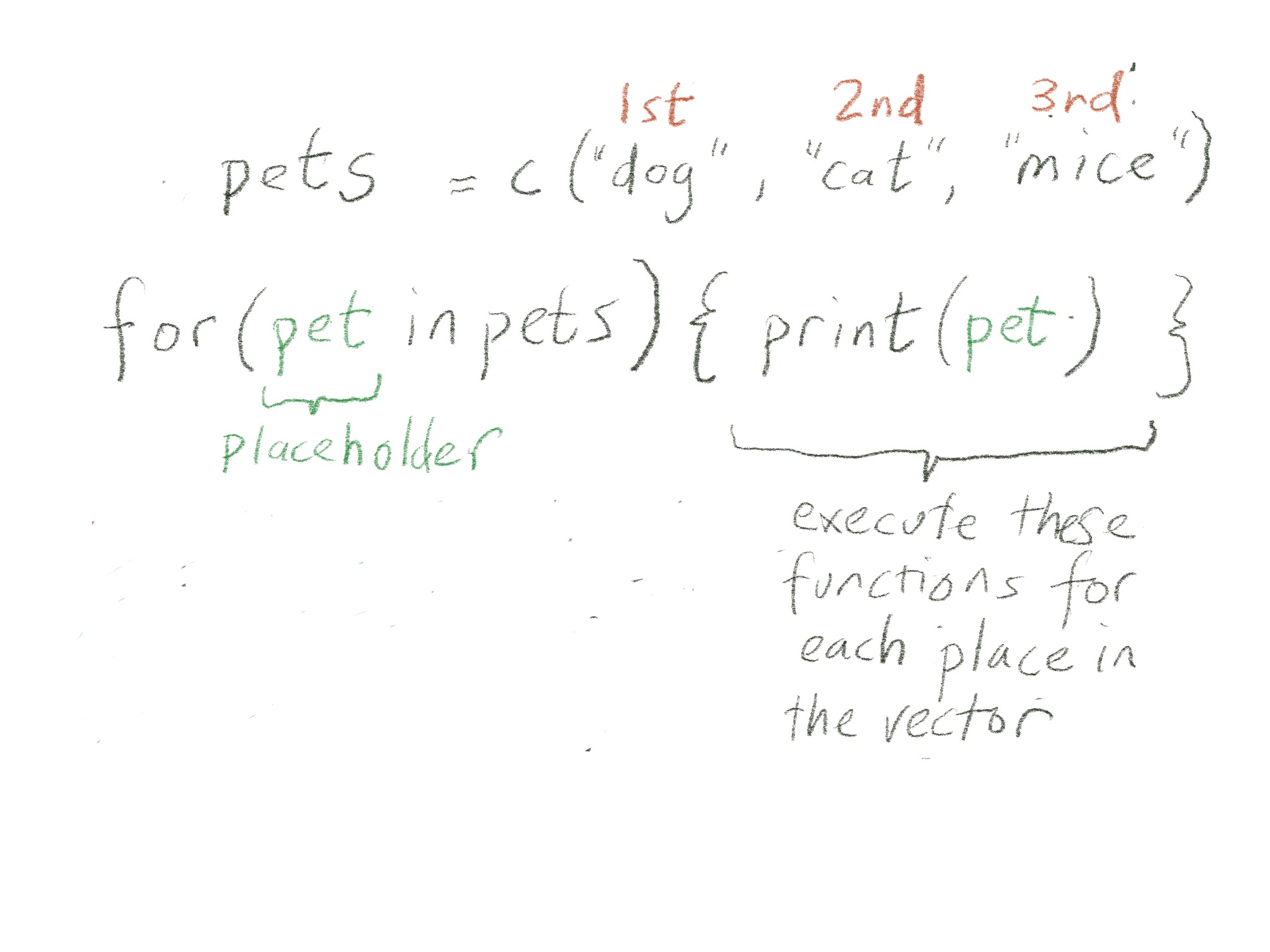
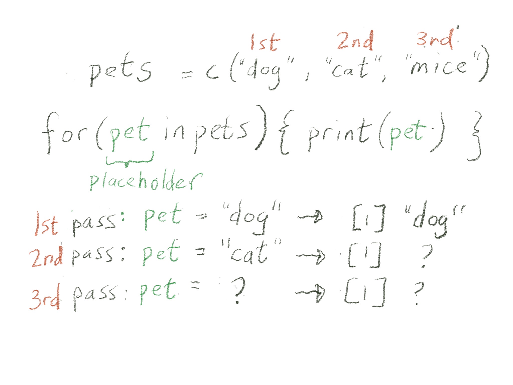
[1]  0.03040693 -1.26680178
# for each index in the vector of pets, do the thing inside {}
pets <- c("dog", "cat", "mice")

for(index in pets) {
  print(index)
}
[1] "dog"
[1] "cat"
[1] "mice"
  • We can change the name of the index:
# for each index in the vector of pets, do the thing inside {}
pets <- c("dog", "cat", "mice")

for(pet in pets) {
  print(pet)
}
[1] "dog"
[1] "cat"
[1] "mice"
  • A visual explanation (via Ted Laderas)


3.2 Saving for() loop output

  • What does this for() loop do?
pets <- c("dog", "cat", "mice")

for(pet in pets){
  mypet <- paste("meike's", pet)
  print(mypet)
}
[1] "meike's dog"
[1] "meike's cat"
[1] "meike's mice"
  • Note that the last iteration of mypet is also saved as an object outside of the loop (into the global environment):
mypet
[1] "meike's mice"
  • But how do we capture all of the output the for() loop creates?
    • We need to save it explicitly as a vector or list.
  • Save all of the output the for() loop creates as a vector
# make an empty vector (initialize)
all_my_pets <- c()

for(pet in pets){
  mypet <- paste("meike's", pet)
  
  # add the new variable mypet to the end of the vector all_my_pets
  all_my_pets <- c(all_my_pets, mypet)
}

all_my_pets
[1] "meike's dog"  "meike's cat"  "meike's mice"
  • What happens when you run the for() loop multiple times without initializing all_my_pets?

  • We know all_my_pets is a vector.

    • What does it contain?
    • What is its length?

3.3 Challenge 2

  • The toy example below has vectors for
    • miles per gallon readings for different cars and
    • corresponding number of miles driven per day.
  • The for() loop calculates the number of gallons (ng) used by each car.
  1. Adapt the code below to save the output as a vector of number of gallons driven for each car.
  2. Using the vector created in part 1, calculate the total number of gallons used.
cars_mpg <- c(20, 30, 44.2, 10)
cars_miles <- c(10, 1, 50, 10)

# modify the for loop to save output as a vector:
for(index in seq_along(cars_mpg)) {
  ng <- cars_miles[index] / cars_mpg[index]
  print(ng)
}
[1] 0.5
[1] 0.03333333
[1] 1.131222
[1] 1

How many total gallons of gas did the cars use?

3.4 for() loops with lists

We can also iterate for() loops over lists.

my_list <- list(cat_names = c("Morris", "Julia"), 
                hedgehog_names = "Spiny", 
                dog_names = c("Rover", "Spot", "Kitty"),
                cat_ages = c(10,7))
  • Print the length of each list item
for(index in my_list) {
  length(index) %>% print()
}
[1] 2
[1] 1
[1] 3
[1] 2
  • Print the first element of each list
for(index in my_list) {
  index[[1]] %>% print()
}
[1] "Morris"
[1] "Spiny"
[1] "Rover"
[1] 10

3.5 (Bonus content) Iteration over the length of the vector or list

  • It’s also common to index over the numeric vector from 1 to the length of the list or vector:
pets # reminder what pets looks like
[1] "dog"  "cat"  "mice"
for(index in 1:length(pets)) {
  str_to_upper(pets[index]) %>% print()
}
[1] "DOG"
[1] "CAT"
[1] "MICE"
for(index in 1:length(my_list)) {
  print(index)
  print(my_list[[index]])
}
[1] 1
[1] "Morris" "Julia" 
[1] 2
[1] "Spiny"
[1] 3
[1] "Rover" "Spot"  "Kitty"
[1] 4
[1] 10  7
for(index in 1:length(my_list)) {
  myelement <- my_list[[index]]
  gg <- glue("The length of element {index} is: {length(myelement)}")
  print(gg)
}
The length of element 1 is: 2
The length of element 2 is: 1
The length of element 3 is: 3
The length of element 4 is: 2

4 purrr: no need for for loops 🥳

4.1 Motivation for purrr

  • for() loops can indeed be useful, but they have their pros and cons
  • Pros:
    • Classic programming approach, easy to understand since each step is written out in order of operation (easier to teach, first!)
    • Easy to adapt
    • Somewhat easy to debug
  • Cons:
    • Can become complex quickly, and therefore messy to read
    • Require creating empty vectors and/or appending output in somewhat clunky way
    • Don’t fit “nicely” inside other functions or pipelines

4.2 purrr::map()

Enter the purrr package and map().

  • purrr::map() lets us apply a function to each element of a list.
  • It will always return a list with the number of elements that is the same as the list we input it with.
  • Each slot of the returned list will contain the output of the functions applied to each element of the input list.
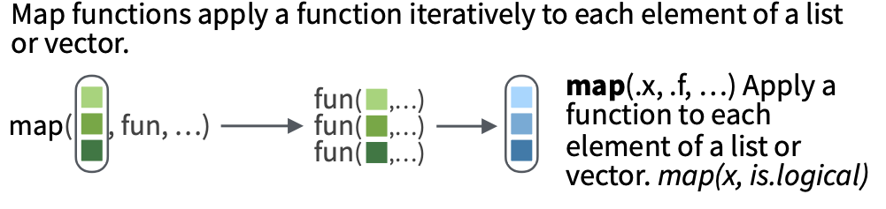
  • The way to read a map() statement is:

map(.x = LIST_OBJECT, .f = FUNCTION_TO_APPLY)

  • Let’s make a function to return the first element of the input vector:
get_first_element <- function(input_vec){
  return(input_vec[1])
}
  • We can apply this function to each element of a list, if the list contains vectors.
    • This is usually easiest if the list is homogeneous,
    • but this specific function can work for heterogeneous lists containing different kinds of vectors as well.
  • The for loop way is similar to the for loop where we printed the first element of the list on a previous slide:
# create my list
my_list <- list(cat_names = c("Morris", "Julia"), 
                hedgehog_names = "Spiny", 
                dog_names = c("Rover", "Spot", "Kitty"),
                cat_ages = c(10,7))

# apply get_first_element to each element of my_list and save the output:

# create empty list
list_output <- list()

# for loop along the length of my list (in this case, 4)
for(index in 1:length(my_list)) {
  
  # print out the index just so we can see what index is
  print(index)
  
  # in the index'th slot, put in the first element of this list
  list_output[[index]] <- get_first_element(my_list[[index]])
}
[1] 1
[1] 2
[1] 3
[1] 4
# print out the result
list_output
[[1]]
[1] "Morris"

[[2]]
[1] "Spiny"

[[3]]
[1] "Rover"

[[4]]
[1] 10
  • That was….not simple.
  • But purrr::map() gives us a much simpler way!
  • First let’s think about what the for loop was doing,
    • with a more straightforward approach,
    • but one that does not scale well:
# apply the function directly to each list element one by one
list_output_by_hand <-
  list(
    get_first_element(my_list[[1]]),
    get_first_element(my_list[[2]]),
    get_first_element(my_list[[3]]),
    get_first_element(my_list[[4]])
  )

list_output_by_hand
[[1]]
[1] "Morris"

[[2]]
[1] "Spiny"

[[3]]
[1] "Rover"

[[4]]
[1] 10
# identical to output from for loop:
# list_output
  • Notice how we were applying the function to each element of the list,
    • one at a time, until we ran out of list elements?
  • purrr::map() does this automatically, without writing out the function 4 (or many more) times.
  • The function map() usually takes two inputs:
    • the list to process
    • the function to process the list items with

map(.x = LIST_OBJECT, .f = FUNCTION_TO_APPLY)

  • Here’s the previous example using map() instead of using a for loop.
new_list <- map(.x = my_list, 
                .f = get_first_element)
new_list
$cat_names
[1] "Morris"

$hedgehog_names
[1] "Spiny"

$dog_names
[1] "Rover"

$cat_ages
[1] 10
  • We have the same output as above using a for loop,

    • but we even got to keep the original list names!
  • Note that we don’t call get_first_element() with the parentheses - (similar to how we use functions by name in across() and/or summarize())

  • We can also leave out the argument names for map() if we like:

new_list <- map(my_list, get_first_element)
new_list
$cat_names
[1] "Morris"

$hedgehog_names
[1] "Spiny"

$dog_names
[1] "Rover"

$cat_ages
[1] 10
  • By default, map() returns the results of your functions to a list.

  • purrr::map() will work on lists or vectors or data frames.

    • We’re focusing on lists and vectors as input for now,
    • because we have other ways of iterating across data frames (summarize() and mutate(), for example), and
    • I don’t want to add too much confusion.

4.3 Challenge 3

  • Use map() to return the length of each of the elements in my_list.
    • Remember to not put the () after the function name.
# switch eval to TRUE

my_list <- list(cat_names = c("Morris", "Julia"), 
                hedgehog_names = "Spiny", 
                dog_names = c("Rover", "Spot", "Kitty"),
                cat_ages = c(10,7))


my_lengths <- map(   )
my_lengths

4.4 Passing in multiple parameters

  • When using a function such as mean, you might need to specify an argument for the function, such as na.omit=TRUE.
my_list2 <- list(vec1 = c(10, 133, 1, NA), 
                 vec2 = c(11, 12, NA, 4), 
                 vec3 = c(1, 5, NA, 4, 100, 22)
)

# what happens without na.omit=TRUE?
map(.x = my_list2, .f = mean)
$vec1
[1] NA

$vec2
[1] NA

$vec3
[1] NA
  • How do we do we specify the function’s arguments?
    • Very similar to how we did this in across:
map(.x = my_list2, 
    .f = ~ mean(.x, na.rm=TRUE))
$vec1
[1] 48

$vec2
[1] 9

$vec3
[1] 26.4

4.5 Tidyverse way

We can also use the pipe with map():

my_list %>%
  map(get_first_element)
$cat_names
[1] "Morris"

$hedgehog_names
[1] "Spiny"

$dog_names
[1] "Rover"

$cat_ages
[1] 10

Meike’s favorite map() example:

# can be done with is.character as well
# penguins doesn't have character variables

penguins %>% select(where(is.factor)) %>% 
  map(tabyl)
$species
   .x[[i]]   n   percent
    Adelie 152 0.4418605
 Chinstrap  68 0.1976744
    Gentoo 124 0.3604651

$island
   .x[[i]]   n   percent
    Biscoe 168 0.4883721
     Dream 124 0.3604651
 Torgersen  52 0.1511628

$sex
 .x[[i]]   n    percent valid_percent
  female 165 0.47965116     0.4954955
    male 168 0.48837209     0.5045045
    <NA>  11 0.03197674            NA

4.6 Help?! More on purrr iteration

The goal of using purrr functions instead of for loops is to allow you to break common list manipulation challenges into independent pieces:

  1. How can you solve the problem for a single element of the list? Once you’ve solved that problem, purrr takes care of generalising your solution to every element in the list.
  2. If you’re solving a complex problem, how can you break it down into bite-sized pieces that allow you to advance one small step towards a solution? With purrr, you get lots of small pieces that you can compose together with the pipe.

This structure makes it easier to solve new problems. It also makes it easier to understand your solutions to old problems when you re-read your old code.

5 purrr::map() with data frames

  • So far, we have used purrr::map() on a variety of simple lists.
  • Now we’re going to take a list of data.frames and use map() and friends of map() to do something to each data frame in the list.

5.1 Two map() examples

We’re going to explore two examples of using map().

  • First example:
    1. Write a function to run a statistical test on a data frame.
    2. Use map() to apply that function to a list of data frames.
  • Second example (next class):
    1. Take a data.frame, and split it into smaller data.frames in a list.
    2. Write a function that works on one of the slots in the list. In this case, we’ll be building a linear model.
    3. Use map() to apply that function to each of the smaller data.frames in our list
    4. Get the linear model results out and aggregate our results using a data.frame

5.2 Example 1

  • Note that the data being read in are in the Part 8 folder!!
lusc_data <- read_csv(here::here("part8", "data", "tumor", "LUSC.csv"))
meso_data <- read_csv(here::here("part8", "data", "tumor", "MESO.csv"))
prad_data <- read_csv(here::here("part8", "data", "tumor", "PRAD.csv"))
read_data <- read_csv(here::here("part8", "data", "tumor", "READ.csv"))
  • Create a list of all the tumor data sets:
my_data_list <- list("LUSC" = lusc_data, 
               "READ" = read_data, 
               "PRAD" = prad_data, 
               "MESO" = meso_data)
  • Create a t-test function that
    • tests the difference in mean age at diagnosis
    • between vital status
    • and tidy the output
my_ttest <- function(mydata) {
  t.test(age_at_diagnosis ~ vital_status, 
         data = mydata) %>%
    tidy()
}

# apply my_ttest to one dataset:
my_ttest(lusc_data)
# A tibble: 1 × 10
  estimate estimate1 estimate2 statistic p.value parameter conf.low conf.high
     <dbl>     <dbl>     <dbl>     <dbl>   <dbl>     <dbl>    <dbl>     <dbl>
1    -736.    24431.    25166.     -2.60 0.00948      467.   -1290.     -181.
# ℹ 2 more variables: method <chr>, alternative <chr>
  • Use map() to apply the t-test function we created to each dataset in the list:
# Apply function to each element of list.
# Note the input/argument needs to be a data frame with the specified columns
tmpout <- map(.x = my_data_list, 
              .f = my_ttest)
tmpout
$LUSC
# A tibble: 1 × 10
  estimate estimate1 estimate2 statistic p.value parameter conf.low conf.high
     <dbl>     <dbl>     <dbl>     <dbl>   <dbl>     <dbl>    <dbl>     <dbl>
1    -736.    24431.    25166.     -2.60 0.00948      467.   -1290.     -181.
# ℹ 2 more variables: method <chr>, alternative <chr>

$READ
# A tibble: 1 × 10
  estimate estimate1 estimate2 statistic p.value parameter conf.low conf.high
     <dbl>     <dbl>     <dbl>     <dbl>   <dbl>     <dbl>    <dbl>     <dbl>
1   -2476.    23312.    25788.     -3.02 0.00445      39.7   -4135.     -816.
# ℹ 2 more variables: method <chr>, alternative <chr>

$PRAD
# A tibble: 1 × 10
  estimate estimate1 estimate2 statistic p.value parameter conf.low conf.high
     <dbl>     <dbl>     <dbl>     <dbl>   <dbl>     <dbl>    <dbl>     <dbl>
1    -405.    22472.    22877.    -0.422   0.683      9.25   -2571.     1760.
# ℹ 2 more variables: method <chr>, alternative <chr>

$MESO
# A tibble: 1 × 10
  estimate estimate1 estimate2 statistic p.value parameter conf.low conf.high
     <dbl>     <dbl>     <dbl>     <dbl>   <dbl>     <dbl>    <dbl>     <dbl>
1    -949.    22381.    23330.    -0.842   0.412      15.9   -3341.     1442.
# ℹ 2 more variables: method <chr>, alternative <chr>
# str(tmpout)

5.3 Challenge 4

  • Create a similar function as my_ttest above that fits a linear regression instead of a t-test with the same outcome/group variables, and apply to the list of data sets using map().

6 Other map output types

  • By default, map() takes a list as an input and returns a list (named, if input is named).
  • However, often it’s useful to have one data frame or tibble as output.

6.1 Data frame output

  • Recall that tmpout is the output from applying map() to our custom function my_ttest.
  • We can use the function list_rbind() to convert a list of data frames/tibbles to one tibble.
  • Use the argument names_to to create a column that contains the original names of the list elements so that we can tell which dataset the output came from.
list_rbind(tmpout, names_to = "data_source") %>% 
  gt()
data_source estimate estimate1 estimate2 statistic p.value parameter conf.low conf.high method alternative
LUSC -735.5727 24430.75 25166.33 -2.6049935 0.009480368 467.490634 -1290.445 -180.7006 Welch Two Sample t-test two.sided
READ -2475.6902 23312.27 25787.96 -3.0162774 0.004447789 39.721988 -4134.904 -816.4769 Welch Two Sample t-test two.sided
PRAD -405.3397 22471.96 22877.30 -0.4216618 0.682899217 9.253084 -2570.898 1760.2187 Welch Two Sample t-test two.sided
MESO -949.3981 22380.62 23330.01 -0.8418847 0.412320094 15.921484 -3340.986 1442.1896 Welch Two Sample t-test two.sided
  • map_df() is a superseded purrr function that returns a data frame.
map_df(.x = my_data_list, 
       .f = my_ttest)
# A tibble: 4 × 10
  estimate estimate1 estimate2 statistic p.value parameter conf.low conf.high
     <dbl>     <dbl>     <dbl>     <dbl>   <dbl>     <dbl>    <dbl>     <dbl>
1    -736.    24431.    25166.    -2.60  0.00948    467.     -1290.     -181.
2   -2476.    23312.    25788.    -3.02  0.00445     39.7    -4135.     -816.
3    -405.    22472.    22877.    -0.422 0.683        9.25   -2571.     1760.
4    -949.    22381.    23330.    -0.842 0.412       15.9    -3341.     1442.
# ℹ 2 more variables: method <chr>, alternative <chr>
  • It essentially row binds the list output together.
  • See the help file (?map_df) for the reasons it was put into lifecycle superseded.
  • It is now recommended to use map() together with list_rbind() instead.

6.2 Type-specific maps

Note that there are type-specific maps that return a vector of numeric values or whatever type you expect, such as

  • map_int() - returns an integer vector
    • your function that you map should return an integer
  • map_chr() - function should return a character vector
    • your function should return a character
  • map_dbl() - function should return a double (decimal) vector
    • your function should return a double

The main difference between these is that they are strict: if you function doesn’t return the desired data type, it will return an error.

Recall my_list:

my_list
$cat_names
[1] "Morris" "Julia" 

$hedgehog_names
[1] "Spiny"

$dog_names
[1] "Rover" "Spot"  "Kitty"

$cat_ages
[1] 10  7
  • Examples that return an integer vector:
map_int(my_list, length)
     cat_names hedgehog_names      dog_names       cat_ages 
             2              1              3              2 
map_int(my_data_list, nrow)
LUSC READ PRAD MESO 
 504  172  500   87 

Examples that return a character vector.

  • What’s happening here?
map_chr(my_list, ~paste(.x, collapse = ", "))
           cat_names       hedgehog_names            dog_names 
     "Morris, Julia"              "Spiny" "Rover, Spot, Kitty" 
            cat_ages 
             "10, 7" 
  • What’s going on with this one?
map_chr(my_list, pluck(1))
     cat_names hedgehog_names      dog_names       cat_ages 
      "Morris"        "Spiny"        "Rover"    "10.000000" 

6.3 Challenge 5

1a. Write a function that returns the first column name of a data frame.

1b. Apply this function to each of the data frames in my_data_list using a type-specific map from above.

2a. Write a function that takes a data frame as an argument and returns the first 3 rows. (Hint: remember slice()? or head() or slice_head()?).

2b. Apply this function using map() to my_data_list and return a stacked (row-wise) data frame of the first 3 rows of each element of the list, making sure to save the name of the data frame in a column called source.

7 Motivation for next time: using map() on split or nested data frames

  • Usually we are not working with a list of data frames that we’ve created ourselves.
  • Often, we have one data frame and we want to perform the same operation on subsets of that data frame.

7.1 Example

  • For instance, we have a complete set of smoking/tumor data set in the data smoke_complete.
  • We can perform our t-test
    • on each of the subsets defined by disease
    • by creating a “nested” data frame by disease, and
    • apply map() within mutate() to the sub data sets. - We will go further into this useful method in the next class.
# Note the data are in the part8/data folder!
smoke_complete <- read_csv(here::here("part8", "data", "clinical.csv"))

glimpse(smoke_complete)
Rows: 6,832
Columns: 20
$ primary_diagnosis           <chr> "C34.1", "C34.1", "C34.3", "C34.1", "C34.3…
$ tumor_stage                 <chr> "stage ia", "stage ib", "stage ib", "stage…
$ age_at_diagnosis            <dbl> 24477, 26615, 28171, 27154, 29827, 23370, …
$ vital_status                <chr> "dead", "dead", "dead", "alive", "dead", "…
$ morphology                  <chr> "8070/3", "8070/3", "8070/3", "8083/3", "8…
$ days_to_death               <dbl> 371, 136, 2304, NA, 146, NA, 345, 716, 280…
$ state                       <chr> "live", "live", "live", "live", "live", "l…
$ tissue_or_organ_of_origin   <chr> "C34.1", "C34.1", "C34.3", "C34.1", "C34.3…
$ days_to_birth               <dbl> -24477, -26615, -28171, -27154, -29827, -2…
$ site_of_resection_or_biopsy <chr> "C34.1", "C34.1", "C34.3", "C34.1", "C34.3…
$ days_to_last_follow_up      <dbl> NA, NA, 2099, 3747, NA, 3576, NA, NA, 1810…
$ cigarettes_per_day          <dbl> 10.9589041, 2.1917808, 1.6438356, 1.095890…
$ years_smoked                <dbl> NA, NA, NA, NA, NA, NA, NA, NA, NA, NA, 26…
$ gender                      <chr> "male", "male", "female", "male", "male", …
$ year_of_birth               <dbl> 1936, 1931, 1927, 1930, 1923, 1942, 1953, …
$ race                        <chr> "white", "asian", "white", "white", "not r…
$ ethnicity                   <chr> "not hispanic or latino", "not hispanic or…
$ year_of_death               <dbl> 2004, 2003, NA, NA, 2004, NA, 2005, 2006, …
$ bcr_patient_barcode         <chr> "TCGA-18-3406", "TCGA-18-3407", "TCGA-18-3…
$ disease                     <chr> "LUSC", "LUSC", "LUSC", "LUSC", "LUSC", "L…
my_ttest <- function(mydata) {
  mydata <- mydata %>% mutate(yrs_diagnosis = age_at_diagnosis/365.25)
  t.test(yrs_diagnosis ~ vital_status, data = mydata) %>% tidy()
}

# check function works on one dataset:
smoke_complete %>%
  filter(vital_status %in% c("alive", "dead")) %>% 
  my_ttest()
# A tibble: 1 × 10
  estimate estimate1 estimate2 statistic  p.value parameter conf.low conf.high
     <dbl>     <dbl>     <dbl>     <dbl>    <dbl>     <dbl>    <dbl>     <dbl>
1    -3.32      60.0      63.3     -9.21 5.08e-20     4302.    -4.03     -2.61
# ℹ 2 more variables: method <chr>, alternative <chr>
  • Group the dataset by disease with group_nest()
  • Notice the structure of the grouped tibble!
    • Each row of the tibble is for a different disease’s data.
grouped_smoke <- smoke_complete %>%
  filter(vital_status %in% c("alive", "dead")) %>%
  group_nest(disease) 

grouped_smoke
# A tibble: 15 × 2
   disease                data
   <chr>   <list<tibble[,19]>>
 1 BLCA             [412 × 19]
 2 BRCA           [1,097 × 19]
 3 CESC             [307 × 19]
 4 COAD             [459 × 19]
 5 GBM              [594 × 19]
 6 LGG              [515 × 19]
 7 LUSC           [1,008 × 19]
 8 MESO              [87 × 19]
 9 PRAD             [500 × 19]
10 READ             [170 × 19]
11 SKCM             [470 × 19]
12 STAD             [443 × 19]
13 THYM             [124 × 19]
14 UCEC             [548 × 19]
15 UCS               [57 × 19]
  • Apply map() via a mutate().
  • Notice that each row (disease) has its own t-test output in the last column.
grouped_smoke <- grouped_smoke %>%
  mutate(t_out = map(data, my_ttest))
grouped_smoke
# A tibble: 15 × 3
   disease                data t_out            
   <chr>   <list<tibble[,19]>> <list>           
 1 BLCA             [412 × 19] <tibble [1 × 10]>
 2 BRCA           [1,097 × 19] <tibble [1 × 10]>
 3 CESC             [307 × 19] <tibble [1 × 10]>
 4 COAD             [459 × 19] <tibble [1 × 10]>
 5 GBM              [594 × 19] <tibble [1 × 10]>
 6 LGG              [515 × 19] <tibble [1 × 10]>
 7 LUSC           [1,008 × 19] <tibble [1 × 10]>
 8 MESO              [87 × 19] <tibble [1 × 10]>
 9 PRAD             [500 × 19] <tibble [1 × 10]>
10 READ             [170 × 19] <tibble [1 × 10]>
11 SKCM             [470 × 19] <tibble [1 × 10]>
12 STAD             [443 × 19] <tibble [1 × 10]>
13 THYM             [124 × 19] <tibble [1 × 10]>
14 UCEC             [548 × 19] <tibble [1 × 10]>
15 UCS               [57 × 19] <tibble [1 × 10]>
  • unnest() the grouped t-test output so that the t-test output for all of the diseased is “flat” in one tibble.
  • Specify which columns to unnest with the cols argument.
grouped_smoke %>%
  select(-data) %>%
  unnest(cols = c(t_out)) %>%
  mutate(p.value = scales::label_pvalue()(p.value)) %>% 
  gt()
disease estimate estimate1 estimate2 statistic p.value parameter conf.low conf.high method alternative
BLCA -4.18141011 66.69616 70.87757 -4.13296252 <0.001 407.723029 -6.170253 -2.1925672 Welch Two Sample t-test two.sided
BRCA -2.93049758 58.67507 61.60557 -2.28291008 0.024 189.107325 -5.462645 -0.3983506 Welch Two Sample t-test two.sided
CESC -4.26809399 47.68270 51.95080 -2.12227460 0.036 103.322202 -8.256477 -0.2797109 Welch Two Sample t-test two.sided
COAD -3.84771067 66.53747 70.38518 -2.56572823 0.011 155.986184 -6.809965 -0.8854561 Welch Two Sample t-test two.sided
GBM -3.61490053 55.31546 58.93036 -2.14203361 0.034 136.010467 -6.952234 -0.2775670 Welch Two Sample t-test two.sided
LGG -6.60418948 41.81057 48.41476 -4.63697902 <0.001 192.951960 -9.413275 -3.7951035 Welch Two Sample t-test two.sided
LUSC -2.01388823 66.88776 68.90165 -3.68786423 <0.001 937.087892 -3.085580 -0.9421966 Welch Two Sample t-test two.sided
MESO -2.59931041 61.27479 63.87410 -0.84188467 0.412 15.921484 -9.147121 3.9485000 Welch Two Sample t-test two.sided
PRAD -1.10975952 61.52487 62.63463 -0.42166179 0.683 9.253084 -7.038735 4.8192161 Welch Two Sample t-test two.sided
READ -6.77807046 63.82552 70.60359 -3.01627737 0.004 39.721988 -11.320749 -2.2353919 Welch Two Sample t-test two.sided
SKCM -0.08157551 58.69815 58.77973 -0.05563643 0.956 456.011625 -2.962971 2.7998196 Welch Two Sample t-test two.sided
STAD -1.56574754 65.60611 67.17186 -1.51171531 0.131 384.531147 -3.602175 0.4706797 Welch Two Sample t-test two.sided
THYM -7.48772570 58.12700 65.61472 -1.91421727 0.085 9.803597 -16.227125 1.2516736 Welch Two Sample t-test two.sided
UCEC -4.32697548 63.68563 68.01261 -3.30806084 0.001 125.133543 -6.915662 -1.7382891 Welch Two Sample t-test two.sided
UCS -4.76002738 67.40041 72.16044 -2.12320590 0.038 54.695884 -9.253468 -0.2665864 Welch Two Sample t-test two.sided

8 Post Class Survey

Please fill out the post-class survey.

Your responses are anonymous in that I separate your names from the survey answers before compiling/reading.

You may want to review previous years’ feedback here.

9 Acknowledgements

  • Part 9 is based on the BSTA 505 Winter 2023 course, taught by Jessica Minnier.
    • I made modifications to update the material from RMarkdown to Quarto, and streamlined/edited content for slides.
  • Minnier’s Acknowledgements: