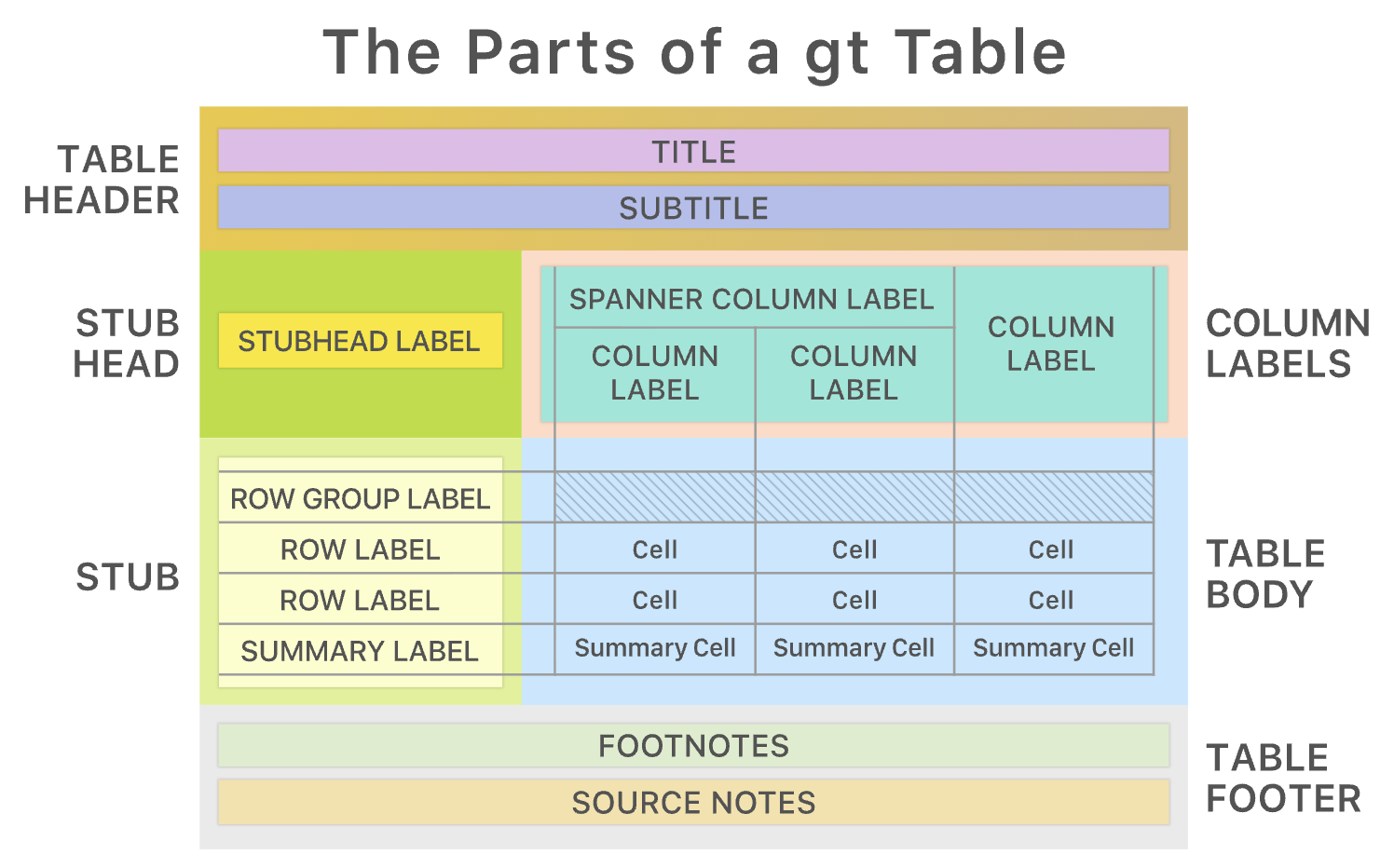
7: Customizing tables, adding and reordering factors, and more ggplot
BSTA 526: R Programming for Health Data Science
2026-02-19
3.3 Add gt() options to tabyl()
- Default
gt() - Important!!!
adorn_title()does not work together withgt()unless the optionplacement = "combined"is included
penguins %>%
  tabyl(species, sex) %>%
  adorn_percentages(denominator = "all") %>%
  adorn_totals(where = c("row", "col")) %>%
  adorn_pct_formatting() %>%
  adorn_ns(position = "front") %>%
  # add title, need placement = "combined" for gt to work
adorn_title(placement = "combined") %>%
# make it fancy html
gt()| species/sex | female | male | NA_ | Total |
|---|---|---|---|---|
| Adelie | 73 (21.2%) | 73 (21.2%) | 6 (1.7%) | 152 (44.2%) |
| Chinstrap | 34 (9.9%) | 34 (9.9%) | 0 (0.0%) | 68 (19.8%) |
| Gentoo | 58 (16.9%) | 61 (17.7%) | 5 (1.5%) | 124 (36.0%) |
| Total | 165 (48.0%) | 168 (48.8%) | 11 (3.2%) | 344 (100.0%) |
- We can use
gtpackage functions to make the table even nicer tab_spanner()is also a prettier and clearer way to add in the name for the column headers instead of usingadorn_title()
penguins %>%
  tabyl(species, sex) %>%
  adorn_percentages(denominator = "all") %>%
  adorn_totals(where = c("row", "col")) %>%
  adorn_pct_formatting() %>%
  adorn_ns(position = "front") %>%
  # specify that species denotes the name of the rows (removes the column label)
  # add line between row names and rest of table
  gt(
    rowname_col = "species") %>%
  # add Species back in as row header
  tab_stubhead(
    label = "Species") %>%
  # add sex label across multiple columns
  tab_spanner(
    label = "Sex",
    columns = c(female, male, `NA_`)
  ) %>%
  # add title
  tab_header(
    title = "Species by sex percentages (counts)",
    subtitle = "Palmer penguin data"
)| Species by sex percentages (counts) | ||||
| Palmer penguin data | ||||
| Species |
Sex
|
Total | ||
|---|---|---|---|---|
| female | male | NA_ | ||
| Adelie | 73 (21.2%) | 73 (21.2%) | 6 (1.7%) | 152 (44.2%) |
| Chinstrap | 34 (9.9%) | 34 (9.9%) | 0 (0.0%) | 68 (19.8%) |
| Gentoo | 58 (16.9%) | 61 (17.7%) | 5 (1.5%) | 124 (36.0%) |
| Total | 165 (48.0%) | 168 (48.8%) | 11 (3.2%) | 344 (100.0%) |
See the very useful vignettes about the gt package, for more.
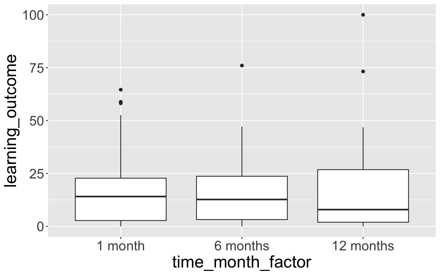
4.3 ggplot boxplot example
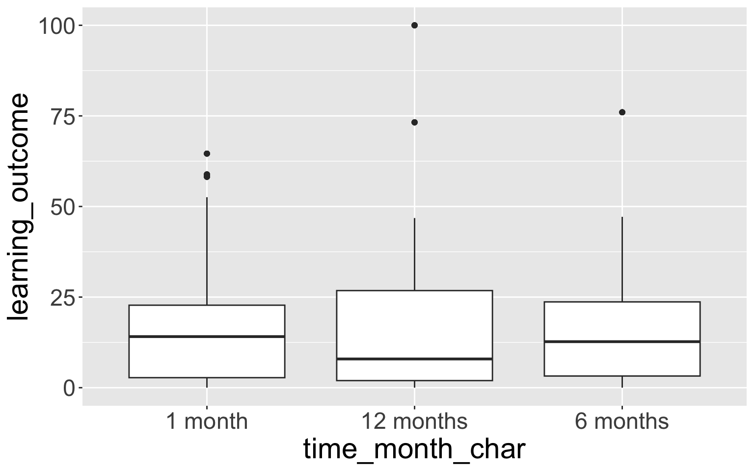
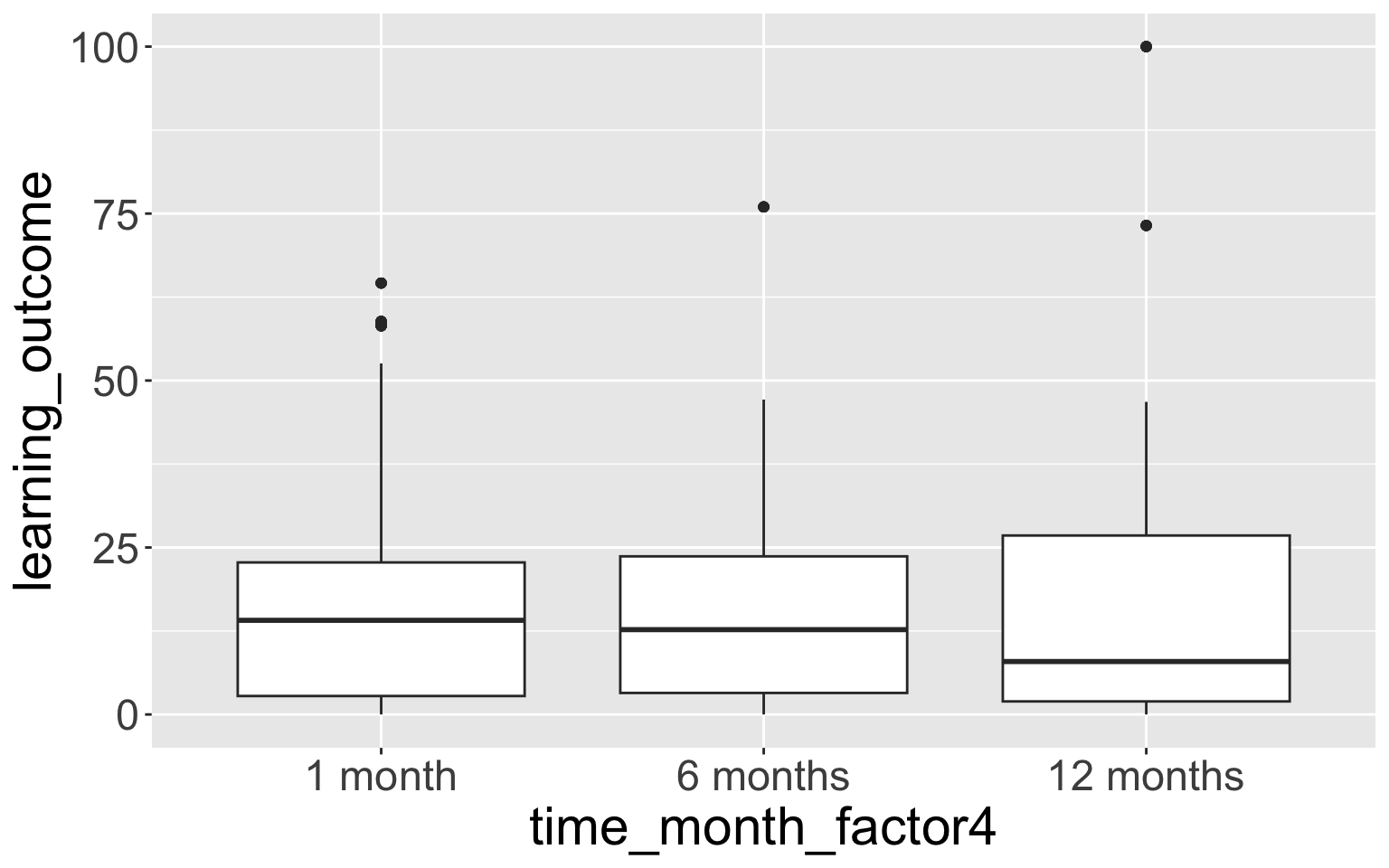
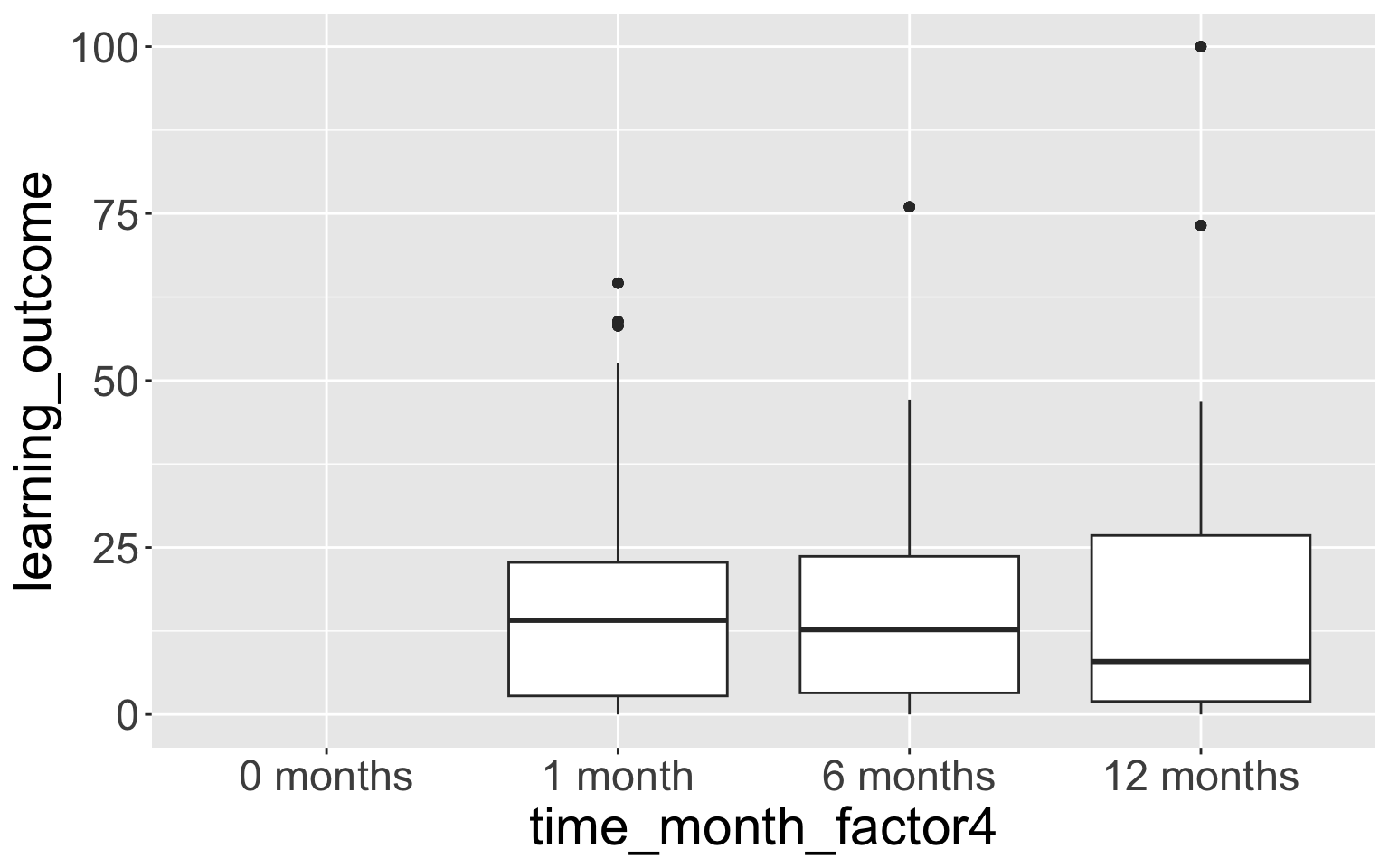
- This doesn’t show the empty time category “0 months”.
- We can fix this with
scale_x_discrete():
- If we want to use the factor as a facet (without adding that extra row of empty data), we can also show an empty level with
drop = FALSEinsidefacet_grid():
# could even add the factor level as a facet
# do not need to add extra row, since we use drop=FALSE
ggplot(mouse_fac,
       aes(x = biomarker_location,
           y = biomarker_value,
           fill = trt)) +
  geom_boxplot() +
  facet_grid(cols = vars(time_month_factor4),
             rows = vars(biomarker_type),
             scales="free_y",
             # WE NEED TO ADD THIS BECAUSE NO DATA
             drop = FALSE) +
  theme_bw() +
  labs(x = "Biomarker Tissue",
       y = "Biomarker Value (pg/mg)",
       fill = "Treatment") +
  ggthemes::scale_fill_tableau()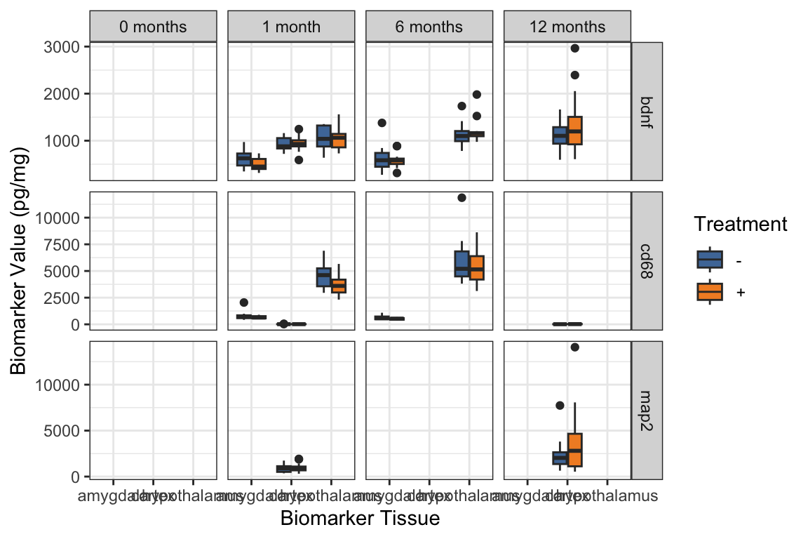
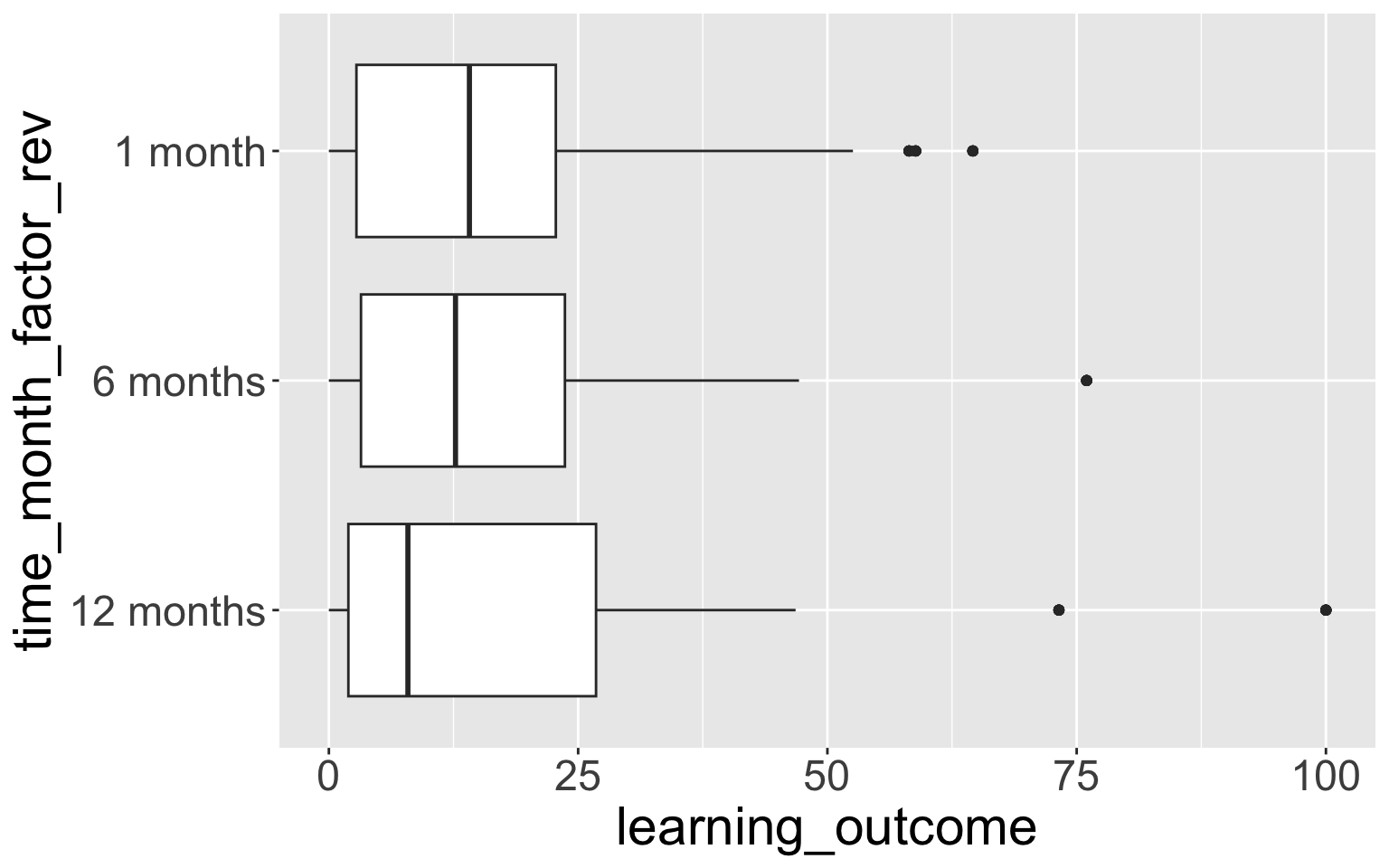
4.4 fct_rev() - reversing the order of a factor
- Very useful when using factors on the y-axis, because the default ordering is first value at the bottom, rather than first value at the top.
# library(forcats)

mouse_fac <- mouse_fac %>%
  mutate(
    time_month_factor_rev = fct_rev(time_month_factor))

# check: compare original & reversed factor vars
mouse_fac %>% tabyl(time_month_factor, time_month_factor_rev) %>%
  adorn_title()
time_month_factor_rev
time_month_factor 12 months 6 months 1 month
1 month 0 0 224
6 months 0 224 0
12 months 224 0 0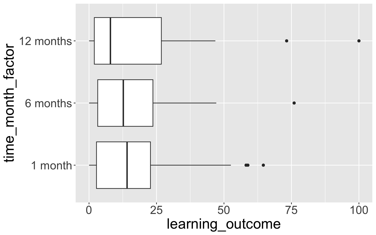
4.5 fct_reorder()
fct_reorder()lets you reorder factors by anothernumericvariable.- Below we reorder the levels of
time_month_factorby the median values ofmirna2at the 3 time points.
- Reorder the levels of
time_month_factorby the median values ofmirna2at the 3 time points.
mouse_fac <- mouse_fac %>%
  mutate(time_month_factor_reorder =
           fct_reorder(time_month_factor, mirna2,
                       .fun = median, na.rm = TRUE))

# check
mouse_fac %>%
  tabyl(time_month_factor_reorder, time_month_factor)
time_month_factor_reorder 1 month 6 months 12 months
6 months 0 224 0
1 month 224 0 0
12 months 0 0 224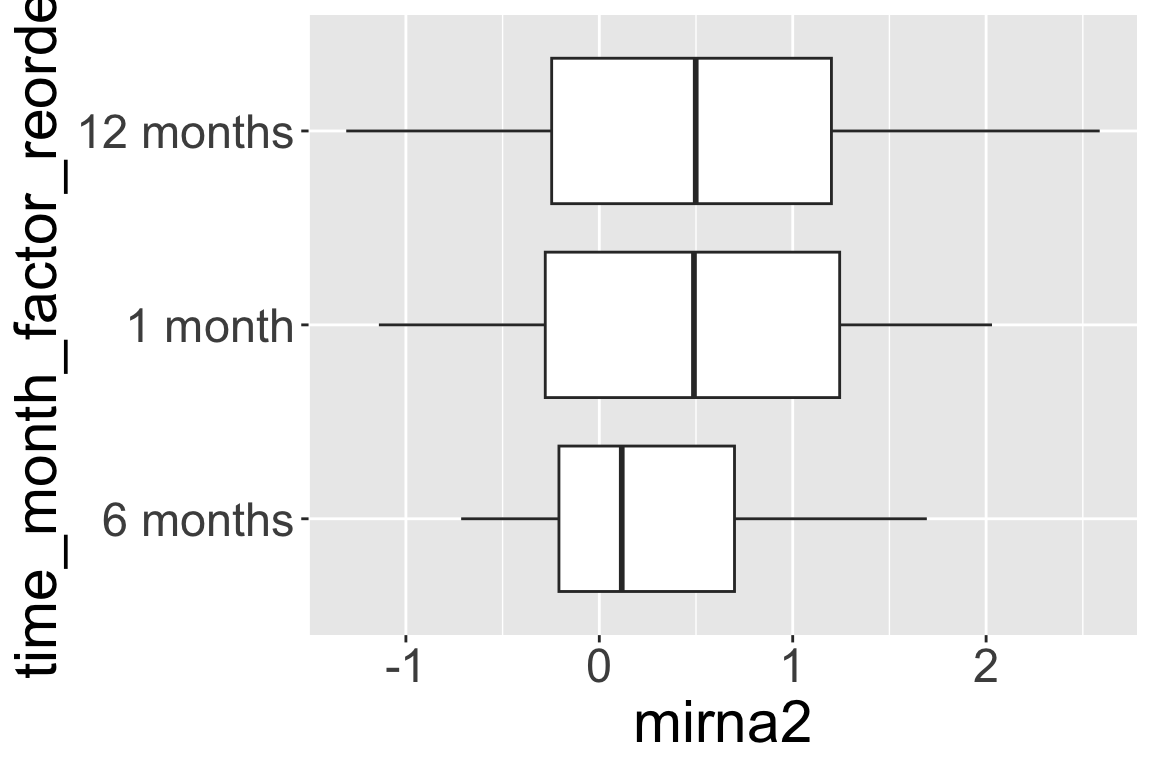
5.1 geom_jitter() & “dodged” boxplots
With small datasets, it is often more informative to show the actual data values, rather than a summary like a boxplot.
We use
geom_jitterto show the data values with random horizontal (or vertical, or both) “jitter” (noise) so they don’t all pile on top of each other.When we have “dodged” boxplots, that is, boxplots side by side based on a fill or color, we need to take special care with the position argument.
Always read the reference/help on these functions for more examples; geom_jitter.
What is wrong with the jittering?
ggplot(mouse_biomarker_long,
       aes(x = biomarker_location,
           y = biomarker_value,
           fill = trt)) +
  geom_boxplot(
    alpha = 0.5,
    outlier.color = NA) +
  geom_jitter(pch = 21) +  # jitter layer
  facet_grid(
    cols = vars(time_month),
    rows = vars(biomarker_type),
    scales = "free_y"
  ) +
  theme_bw() +
  labs(
    x = "Biomarker Tissue",
    y = "Biomarker Value (pg/mg)",
    fill = "Treatment") +
  ggthemes::scale_fill_tableau()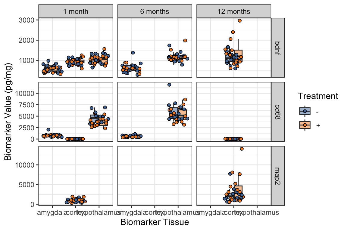
pchis short for plotting character.- What happens if you remove the
pch = 21within thegeom_jitter? - Learn more about different pch symbol options.
- What happens if you remove the
- Adding
position = position_jitterdodge()is a fix for the jittering problem:
ggplot(mouse_biomarker_long,
       aes(x = biomarker_location,
           y = biomarker_value,
           fill = trt)) +
  geom_boxplot(
    alpha = 0.5,
    outlier.color = NA) +
  # note we need position
  # when we have "dodged" boxplots
  geom_jitter(
    pch = 21,
    position = position_jitterdodge()
    ) +
  # This can also be achieved with geom_point:
  # geom_point(pch = 21, position = position_jitterdodge()) +
  facet_grid(
    cols = vars(time_month),
    rows = vars(biomarker_type),
    scales = "free_y"
  ) +
  theme_bw() +
  labs(
    x = "Biomarker Tissue",
    y = "Biomarker Value (pg/mg)",
    fill = "Treatment") +
  ggthemes::scale_fill_tableau()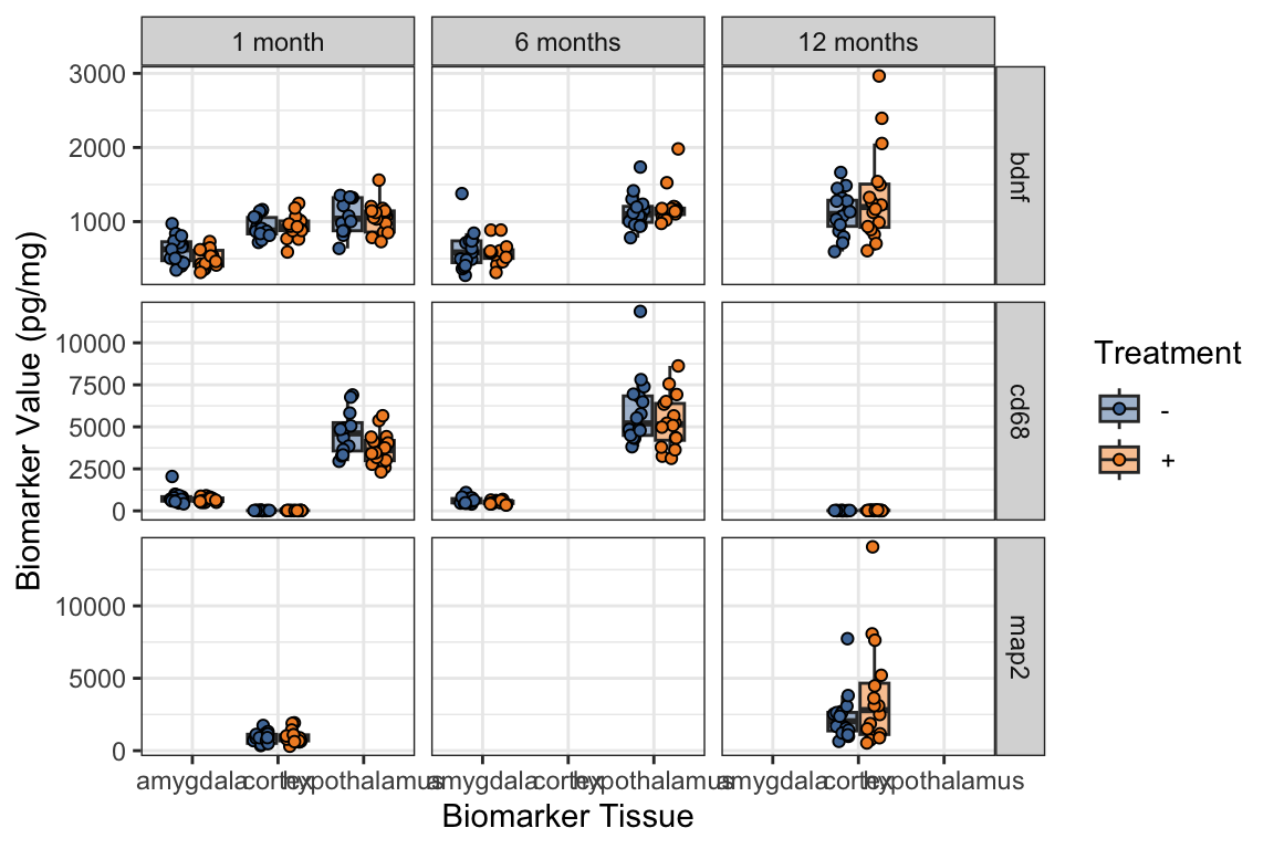
5.2 geom_histogram() with fill
- Below we make histograms of the biomarker values,
- again faceted by the tissue and type.
- We can fill by treatment.
- The default behavior is to stack the histograms for treatment on top of each other,
- so if we want to show overlaid histograms we need to use
position = "identity"argument,- and be sure to choose alpha less than 1 or else you won’t be able to see the two histogram layers.
Note that in facet_grid() the variables are being listed in a different way than what I have showed you previously, which is the same as:
facet_grid(rows = vars(biomarker_type), cols = vars(biomarker_location))
- Histograms with
fill = trt - How to interpret the “filled” histograms?
ggplot(
  # Just show the first time point
  mouse_biomarker_long %>%
    filter(time == "tp1"),
  aes(x = biomarker_value,
      fill = trt)) +
  geom_histogram() +
  facet_grid(
    # the formula way to use facet_grid,
    biomarker_type ~ biomarker_location,
    scales = "free_y") +
  theme_bw() +
  labs(
    x = "Biomarker value (pg/mg)",
    title = "Biomarker distribution (Time Point 1)",
    subtitle = "Stratified by biomarker type and tissue type",
    fill = "Treatment"
  ) +
  ggthemes::scale_fill_tableau()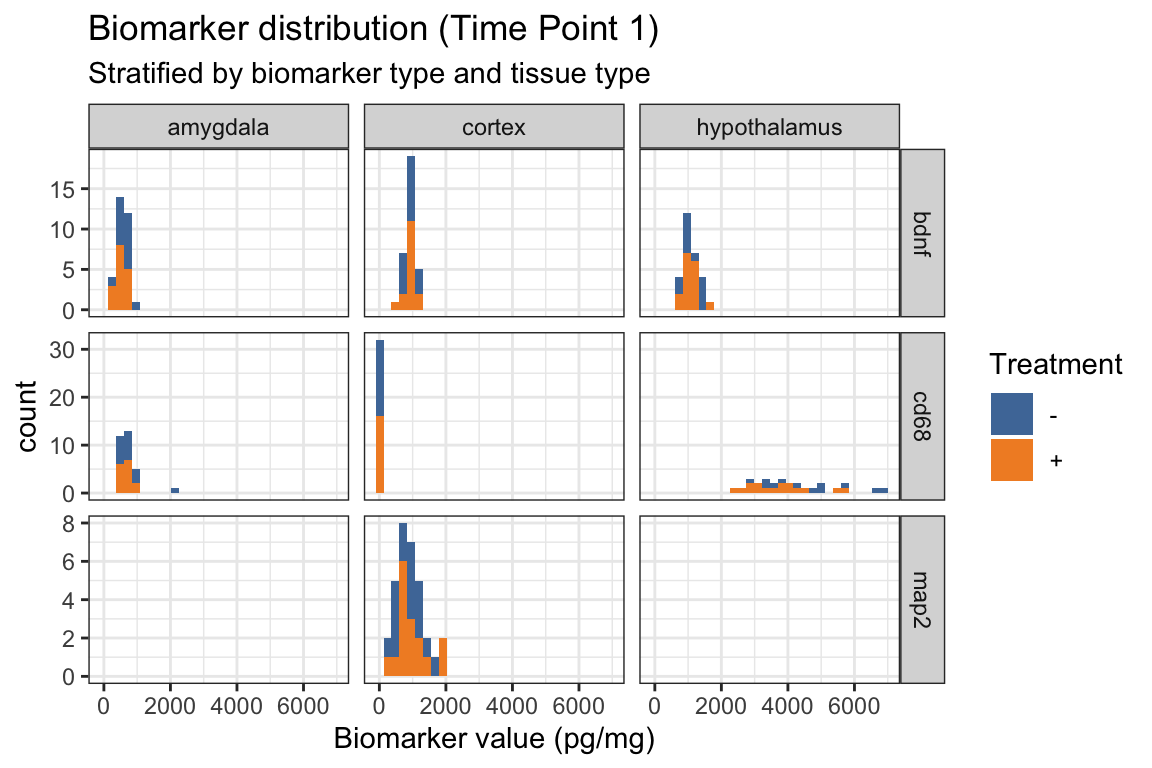
- Below we add
position = "identity"withingeom_histogram() - How does this change the “filled” histograms?
ggplot(
  # Just show the first time point
  mouse_biomarker_long %>%
    filter(time == "tp1"),
  aes(x = biomarker_value,
      fill = trt)) +
  geom_histogram(
    position = "identity"
    ) +
  facet_grid(
    # the formula way to use facet_grid,
    biomarker_type ~ biomarker_location,
    scales = "free_y") +
  theme_bw() +
  labs(
    x = "Biomarker value (pg/mg)",
    title = "Biomarker distribution (Time Point 1)",
    subtitle = "Stratified by biomarker type and tissue type",
    fill = "Treatment"
  ) +
  ggthemes::scale_fill_tableau()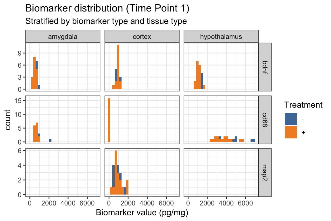
- Below we add
alpha = .4in addition toposition = "identity"withingeom_histogram() - How does this change the “filled” histograms?
ggplot(
  # Just show the first time point
  mouse_biomarker_long %>%
    filter(time == "tp1"),
  aes(x = biomarker_value,
      fill = trt)) +
  geom_histogram(
    alpha = .4,
    position = "identity"
    ) +
  facet_grid(
    # the formula way to use facet_grid,
    biomarker_type ~ biomarker_location,
    scales = "free_y") +
  theme_bw() +
  labs(
    x = "Biomarker value (pg/mg)",
    title = "Biomarker distribution (Time Point 1)",
    subtitle = "Stratified by biomarker type and tissue type",
    fill = "Treatment"
  ) +
  ggthemes::scale_fill_tableau()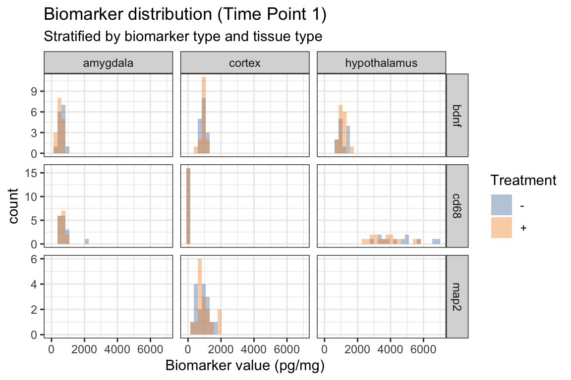
5.3 Scatterplot with different shapes
- New!
shapewithinaes()
ggplot(mouse_biomarker_long %>%
         filter(time=="tp1"),
       aes(x = biomarker_value,
           y = learning_outcome,
           color = trt,
           shape = strain)) +
  geom_point() +
  facet_grid(
    biomarker_type ~ biomarker_location,
    scales = "free_x") +
  theme_bw() +
  labs(
    x = "Biomarker value (pg/mg)",
    y = "Learning Outcome",
    title = "Learning outcome vs biomarkers (Time Point 1)",
    subtitle = "Stratified by biomarker type and tissue type",
    color = "Treatment",
    shape = "Strain") +
  ggthemes::scale_color_tableau()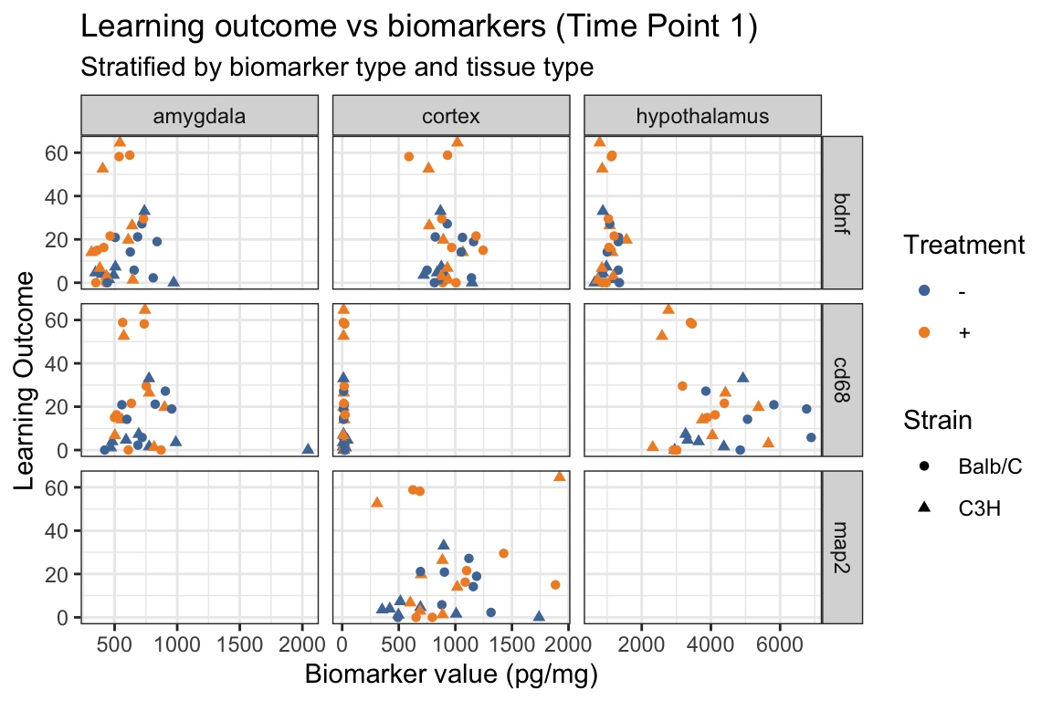
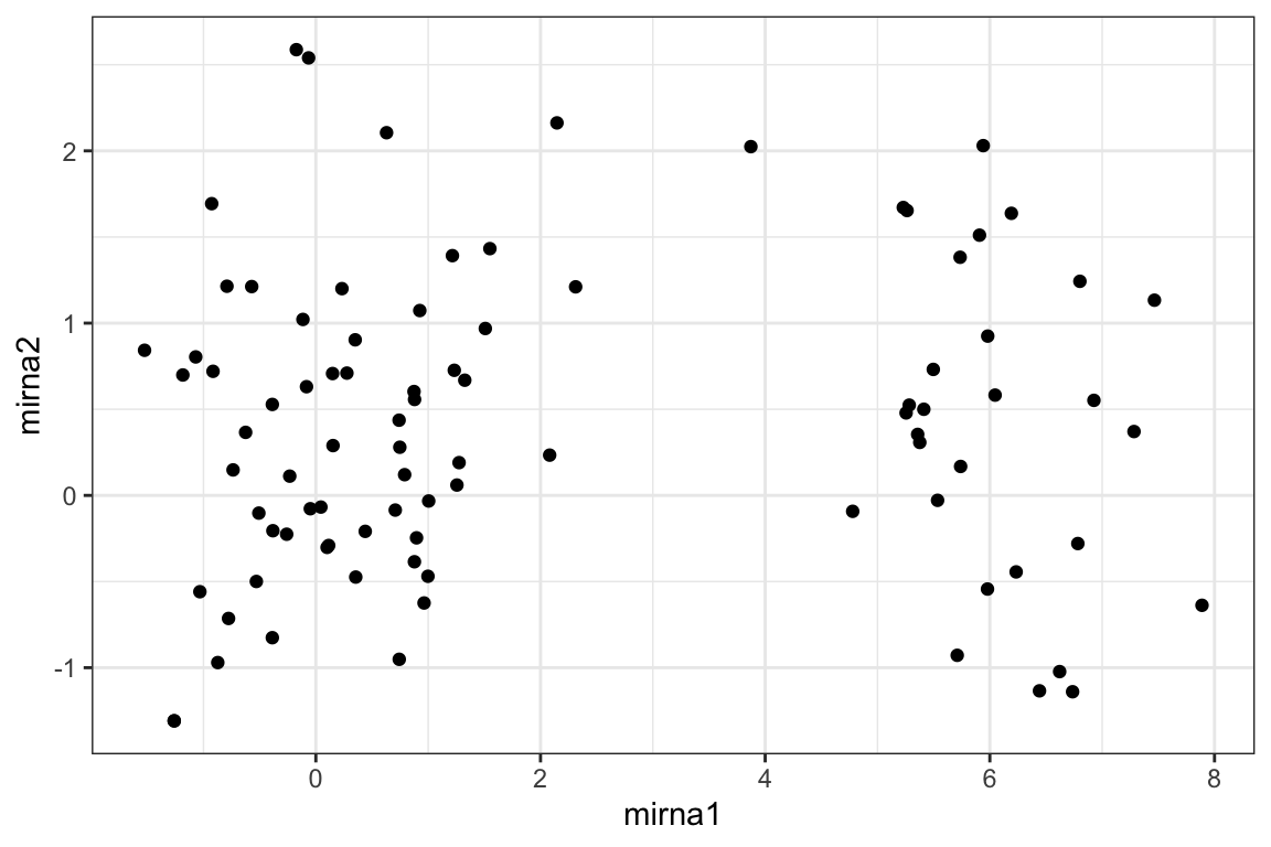
5.4 Challenge 1 (on your own 5 minutes)
What’s going on with tp1?
There seems to be a batch effect in mirna1, can you manipulate this plot to figure out what’s going on?
5.5 geom_line(): scatterplot trajectories
Familiarize yourself with the figure. What does it show?
Also, note how a
facet_wrapwith two variables figure looks different from usingfacet_grid.
ggplot(mouse_data %>%
         arrange(sid,time),
       aes(x = mirna2,
           y = learning_outcome,
           color = trt,
           shape= time_month)
       ) +
  geom_point() +
  facet_wrap(vars(strain, sex)) +
  theme_bw() +
  labs(
    x = "miRNA2 expression",
    y = "Learning Outcome",
    title = "miRNA vs outcome across time points",
    subtitle = "Stratified by 2strain and sex (M/F)") +
  ggthemes::scale_color_tableau()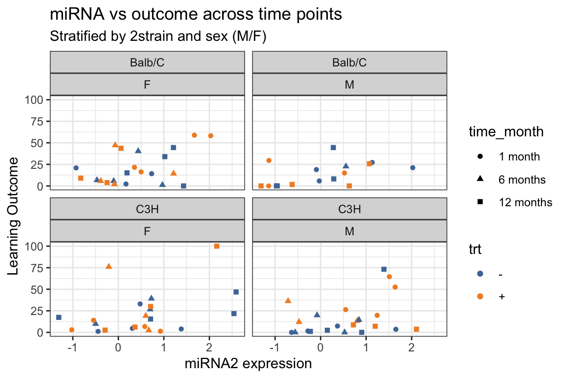
- Add trajectories with
geom_line(). - What trajectories are being shown???
ggplot(mouse_data %>%
         arrange(sid,time),
       aes(x = mirna2,
           y = learning_outcome,
           color = trt,
           shape= time_month)
       ) +
  geom_point() +
  geom_line() +
  facet_wrap(vars(strain, sex)) +
  theme_bw() +
  labs(
    x = "miRNA2 expression",
    y = "Learning Outcome",
    title = "miRNA vs outcome across time points",
    subtitle = "Stratified by 2strain and sex (M/F)") +
  ggthemes::scale_color_tableau()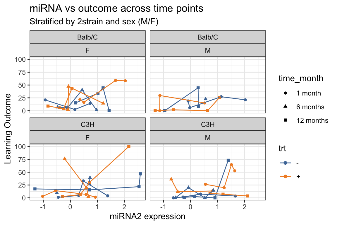
- Add
group = sidwithin theaes(). - How does this change the trajectories?
ggplot(mouse_data %>%
         arrange(sid,time),
       aes(x = mirna2,
           y = learning_outcome,
           color = trt,
           shape= time_month,
           group = sid
           )) +
  geom_point() +
  geom_line() +
  facet_wrap(vars(strain, sex)) +
  theme_bw() +
  labs(
    x = "miRNA2 expression",
    y = "Learning Outcome",
    title = "Trajectory of miRNA vs outcome across time points",
    subtitle = "Stratified by 2strain and sex (M/F)") +
  ggthemes::scale_color_tableau()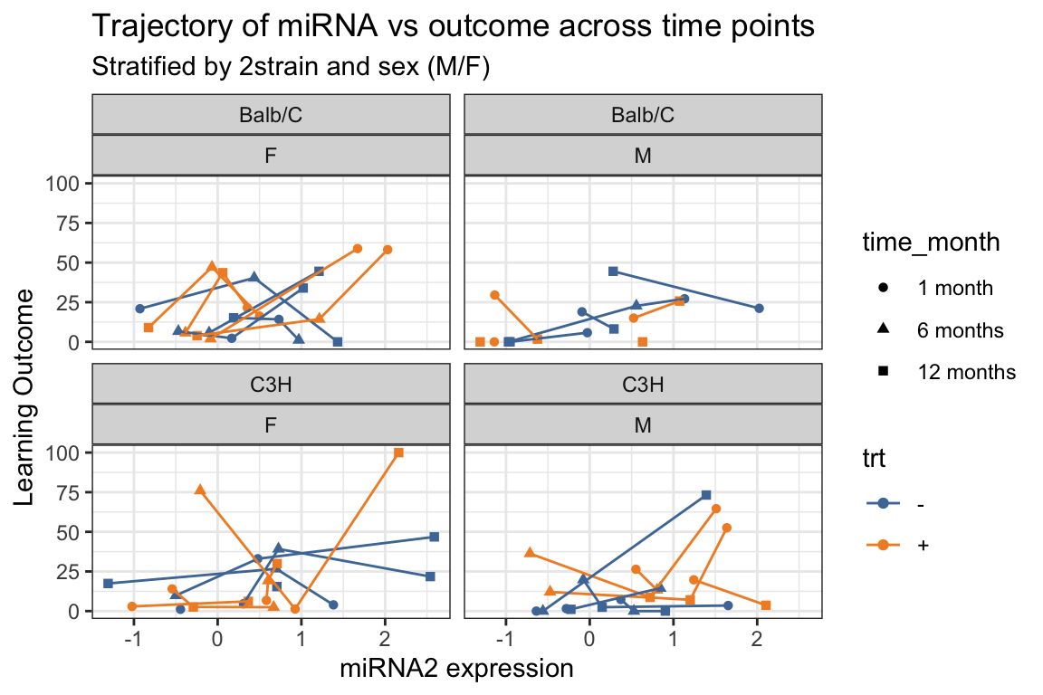
5.6 geom_tile() - with summarized data
geom_tile()is similar to a heatmap, in that the colors of the “tiles” represent numeric values.
Here we use a somewhat complex example.
- Suppose we want to show the difference in mean biomarker between treated and untreated (
trt+minus-) mice,- stratified by biomarker_type, biomarker_location, strain, and sex.
- We first need to create a dataframe that contains the means
- for every combination of the treatment group and stratification variables
- Then we need to take the differences of the two treatment means.
- Calculate mean of biomarker value for each combination of groupings
tmpdata_mean = mouse_biomarker_long %>%
  group_by(biomarker_type,
           biomarker_location,
           trt,
           strain,
           sex) %>%
  summarize(m = mean(biomarker_value, na.rm = TRUE))

tmpdata_mean
# A tibble: 56 × 6
# Groups: biomarker_type, biomarker_location, trt, strain [28]
biomarker_type biomarker_location trt strain sex m
<chr> <chr> <chr> <chr> <chr> <dbl>
1 bdnf amygdala + Balb/C F 588.
2 bdnf amygdala + Balb/C M 559.
3 bdnf amygdala + C3H F 490.
4 bdnf amygdala + C3H M 484.
5 bdnf amygdala - Balb/C F 719.
6 bdnf amygdala - Balb/C M 711.
7 bdnf amygdala - C3H F 499.
8 bdnf amygdala - C3H M 507.
9 bdnf cortex + Balb/C F 1080.
10 bdnf cortex + Balb/C M 1582.
# ℹ 46 more rowspivot_wider()so that we have a+column and a-column that contains those means- Then add a column with the differences
tmpdata_mean_wide = pivot_wider(tmpdata_mean,
                      id_cols = c(biomarker_type,
                                  biomarker_location,
                                  strain,
                                  sex),
                      names_from = trt,
                      values_from = m
                      ) %>%
  mutate(diff = `+` - `-`)

tmpdata_mean_wide
# A tibble: 28 × 7
# Groups: biomarker_type, biomarker_location, strain [14]
biomarker_type biomarker_location strain sex `+` `-` diff
<chr> <chr> <chr> <chr> <dbl> <dbl> <dbl>
1 bdnf amygdala Balb/C F 588. 719. -131.
2 bdnf amygdala Balb/C M 559. 711. -152.
3 bdnf amygdala C3H F 490. 499. -8.51
4 bdnf amygdala C3H M 484. 507. -22.9
5 bdnf cortex Balb/C F 1080. 1005. 75.5
6 bdnf cortex Balb/C M 1582. 1050. 532.
7 bdnf cortex C3H F 974. 1096. -122.
8 bdnf cortex C3H M 920. 937. -16.1
9 bdnf hypothalamus Balb/C F 1092. 1079. 13.6
10 bdnf hypothalamus Balb/C M 1121. 1180. -59.0
# ℹ 18 more rowsFigure using wide data:
ggplot(tmpdata_mean_wide,
       aes(x = biomarker_type,
           y = biomarker_location,
           fill = diff))+
  geom_tile()+
  facet_grid(
    rows = vars(strain),
    cols = vars(sex),
    labeller = labeller(
      sex = label_both,
      strain = label_both)
    ) +
  scale_fill_gradient2(
    low = "purple",
    mid = "white",
    high = "orange") +
  labs(
    x = "Biomarker Type",
    y = "Biomarker Tissue",
    fill = "Difference in Means",
    title = "Difference in mean biomarker values (treated - untreated)"
    ) +
  theme_bw()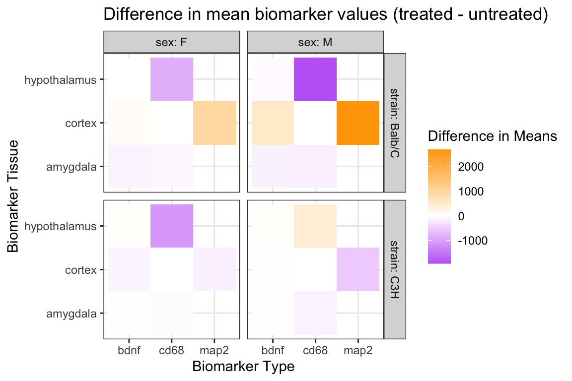
5.7 geom_tile() - with summarize()^2 (more advanced coding)
- Just showing a difference in means may not reflect the varying ranges and variability in the biomarkers.
- Let’s show the difference in means divided by the standard error:
\[\frac{mu_+ - mu_-}{\sqrt{sd^2_+/n_+ + sd^2_-/n_-}}\]
- Instead of using
pivot_wider, we can actually usesummarizea second time- (and we could have done this in the above example as well).
- (similar to before)
tmpdata_summarize = mouse_biomarker_long %>%
  group_by(biomarker_type,
           biomarker_location,
           trt,
           strain,
           sex) %>%
  summarize(m = mean(biomarker_value, na.rm = TRUE),
            se = var(biomarker_value, na.rm = TRUE) /
              length(biomarker_value))

tmpdata_summarize
# A tibble: 56 × 7
# Groups: biomarker_type, biomarker_location, trt, strain [28]
biomarker_type biomarker_location trt strain sex m se
<chr> <chr> <chr> <chr> <chr> <dbl> <dbl>
1 bdnf amygdala + Balb/C F 588. 1768.
2 bdnf amygdala + Balb/C M 559. 3304.
3 bdnf amygdala + C3H F 490. 1440.
4 bdnf amygdala + C3H M 484. 1164.
5 bdnf amygdala - Balb/C F 719. 8177.
6 bdnf amygdala - Balb/C M 711. 464.
7 bdnf amygdala - C3H F 499. 2053.
8 bdnf amygdala - C3H M 507. 3493.
9 bdnf cortex + Balb/C F 1080. 6993.
10 bdnf cortex + Balb/C M 1582. 51650.
# ℹ 46 more rows- In the next bit of code we use a “base R” indexing of a vector.
- Here’s a simple example of this kind of indexing:
- The code below works because we know that there is just
- one value within each group when
trt= “+” and - one value within group when
trt= “-”.
- one value within each group when
- The value of
diffneeds to be a numeric value of length 1, i.e one number.
tmpdata_diff <- tmpdata_summarize %>%
  group_by(biomarker_type,
           biomarker_location,
           strain,
           sex) %>%
  # take m value where trt is + and subtract m value where trt is - and then divide....
  summarize(std_diff = (m[trt == "+"] - m[trt == "-"]) /
              sqrt(se[trt == "+"] + se[trt == "-"])
            )

tmpdata_diff
# A tibble: 28 × 5
# Groups: biomarker_type, biomarker_location, strain [14]
biomarker_type biomarker_location strain sex std_diff
<chr> <chr> <chr> <chr> <dbl>
1 bdnf amygdala Balb/C F -1.31
2 bdnf amygdala Balb/C M -2.47
3 bdnf amygdala C3H F -0.144
4 bdnf amygdala C3H M -0.336
5 bdnf cortex Balb/C F 0.726
6 bdnf cortex Balb/C M 2.25
7 bdnf cortex C3H F -1.24
8 bdnf cortex C3H M -0.150
9 bdnf hypothalamus Balb/C F 0.203
10 bdnf hypothalamus Balb/C M -0.901
# ℹ 18 more rowsggplot(tmpdata_diff,
aes(x = biomarker_type,
y = biomarker_location,
fill = std_diff)) +
geom_tile() +
facet_grid(
rows = vars(strain),
cols = vars(sex),
labeller = labeller(
sex = label_both,
strain = label_both)
) +
scale_fill_gradient2(
low = "purple",
mid="white",
high="orange") +
labs(
x = "Biomarker Type",
y = "Biomarker Tissue",
fill = "Difference in mean/sd",
title = "Difference in mean/sd biomarker values (treated - untreated)") +
theme_bw()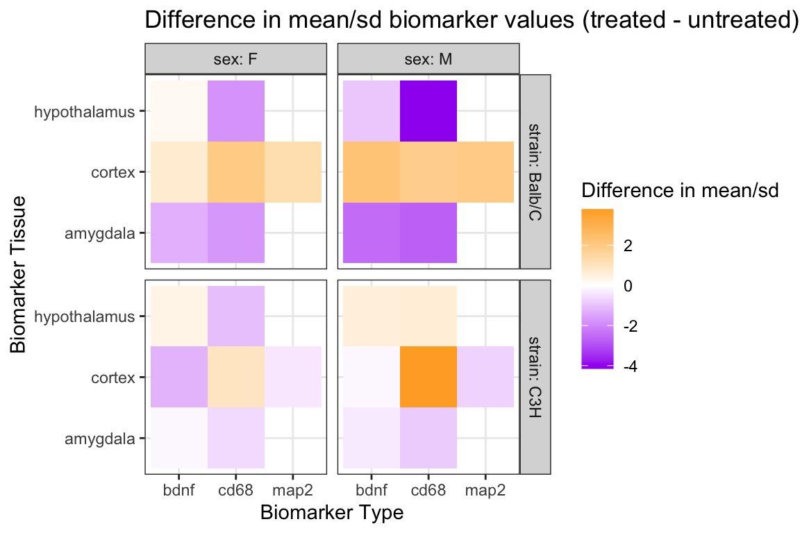
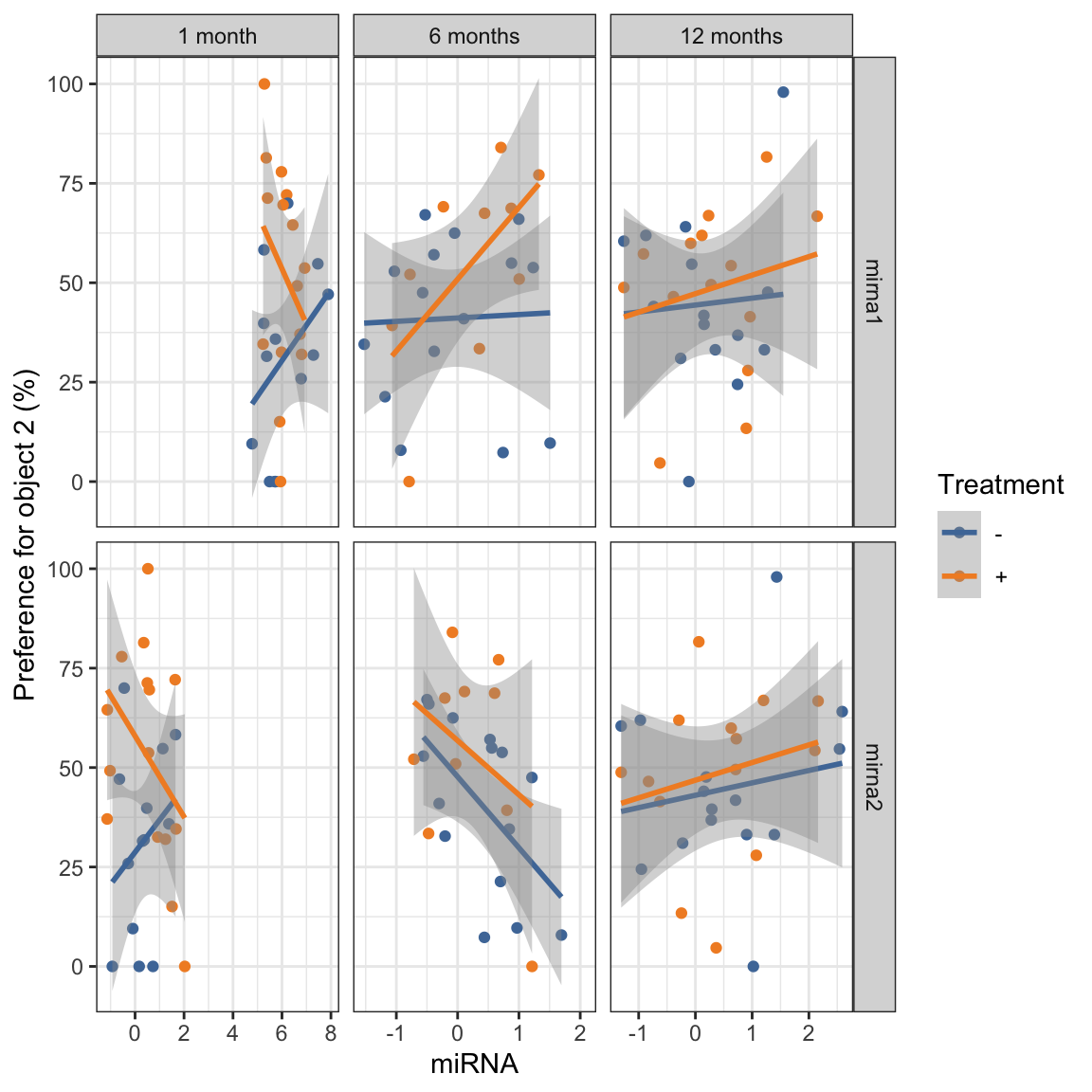
5.8 geom_smooth()
geom_smooth()adds a smoothing curve (or line) to a scatterplot.- The default method is
loess- but we can also show a linear association by using
method = "lm" - to show the least squares fit linear regression line to the data.
- but we can also show a linear association by using
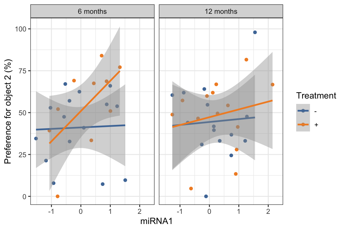
- We can make a longer dataset based on mirna values similar to what we did with the biomarker data, to create one plot of both miRNAs:
# create long mirna data
mouse_mirna_long <- mouse_data %>%
  pivot_longer(cols = starts_with("mir"),
               names_to = "mirna",
               values_to = "mirna_value")

glimpse(mouse_mirna_long)
Rows: 192
Columns: 18
$ sid <dbl> 137, 137, 137, 137, 137, 137, 138, …
$ strain <chr> "C3H", "C3H", "C3H", "C3H", "C3H", …
$ trt <chr> "-", "-", "-", "-", "-", "-", "-", …
$ sex <chr> "M", "M", "M", "M", "M", "M", "M", …
$ time <chr> "tp1", "tp1", "tp2", "tp2", "tp3", …
$ normalized_bdnf_amygdala_pg_mg <dbl> 492.4831, 492.4831, 275.1623, 275.1…
$ normalized_bdnf_cortex_pg_mg <dbl> 720.0173, 720.0173, NA, NA, 871.828…
$ normalized_bdnf_hypothalamus_pg_mg <dbl> NA, NA, 1169.2845, 1169.2845, NA, N…
$ normalized_cd68_amygdala_pg_mg <dbl> 988.9628, 988.9628, 574.0655, 574.0…
$ normalized_cd68_cortex_pg_mg <dbl> 8.393707, 8.393707, NA, NA, NA, NA,…
$ normalized_cd68_hypothalamus_pg_mg <dbl> NA, NA, 6800.870, 6800.870, NA, NA,…
$ normalized_map2_cortex_pg_mg <dbl> 352.9653, 352.9653, NA, NA, 2693.93…
$ learning_outcome <dbl> 3.52, 3.52, 19.81, 19.81, 2.44, 2.4…
$ preference_obj1 <dbl> 41.72205, 41.72205, 37.51387, 37.51…
$ preference_obj2 <dbl> 58.27795, 58.27795, 62.48613, 62.48…
$ time_month <fct> 1 month, 1 month, 6 months, 6 month…
$ mirna <chr> "mirna1", "mirna2", "mirna1", "mirn…
$ mirna_value <dbl> 5.2630200, 1.6536200, -0.0491371, -…ggplot(mouse_mirna_long,
aes(x = mirna_value,
preference_obj2,
color = trt)) +
geom_point() +
geom_smooth(method = "lm") +
ggthemes::scale_color_tableau() +
facet_grid(vars(mirna),
vars(time_month),
scales = "free_x") +
theme_bw() +
labs(
x = "miRNA",
y ="Preference for object 2 (%)",
color = "Treatment")