Rows: 20 Columns: 2
── Column specification ────────────────────────────────────────────────────────
Delimiter: ","
chr (1): Group
dbl (1): Taps

ℹ Use `spec()` to retrieve the full column specification for this data.
ℹ Specify the column types or set `show_col_types = FALSE` to quiet this message.
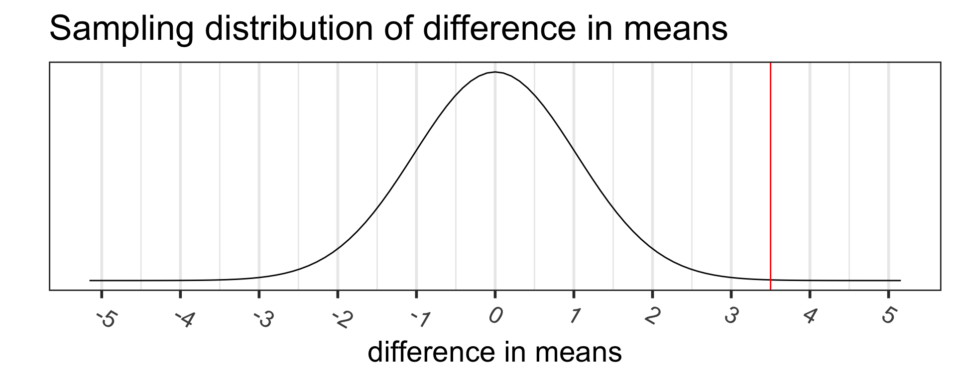
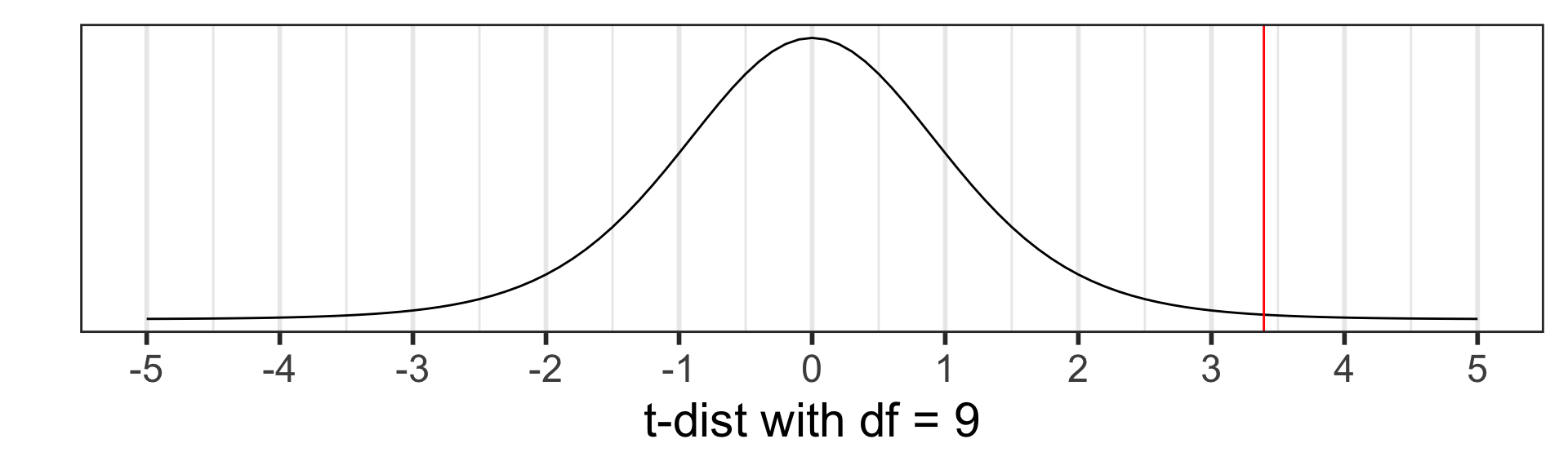
Based on the value of the test statistic, do you think we are going to reject or fail to reject \(H_0\)?
Step “3b”: Assumptions satisfied?
Assumptions:
Independent observations & samples
The observations were collected independently.
In particular, the observations from the two groups were not paired in any meaningful way.
Approximately normal samples or big n’s
The distributions of the samples should be approximately normal
orboth their sample sizes should be at least 30.
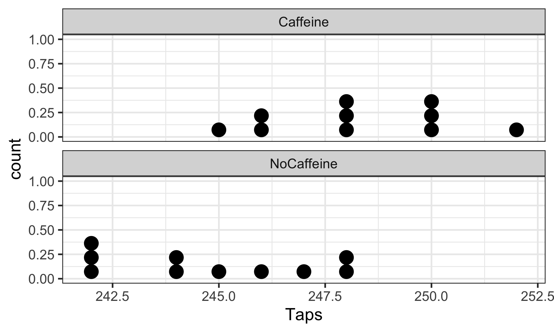
Bin width defaults to 1/30 of the range of the data. Pick better value with
`binwidth`.
Step 4: p-value
The p-value is the probability of obtaining a test statistic just as extreme or more extreme than the observed test statistic assuming the null hypothesis \(H_0\) is true.
There is sufficient evidence that the (population) difference in mean finger taps/min with vs. without caffeine is greater than 0 ( \(p\)-value = 0.004).
More realistic manuscript conclusion:
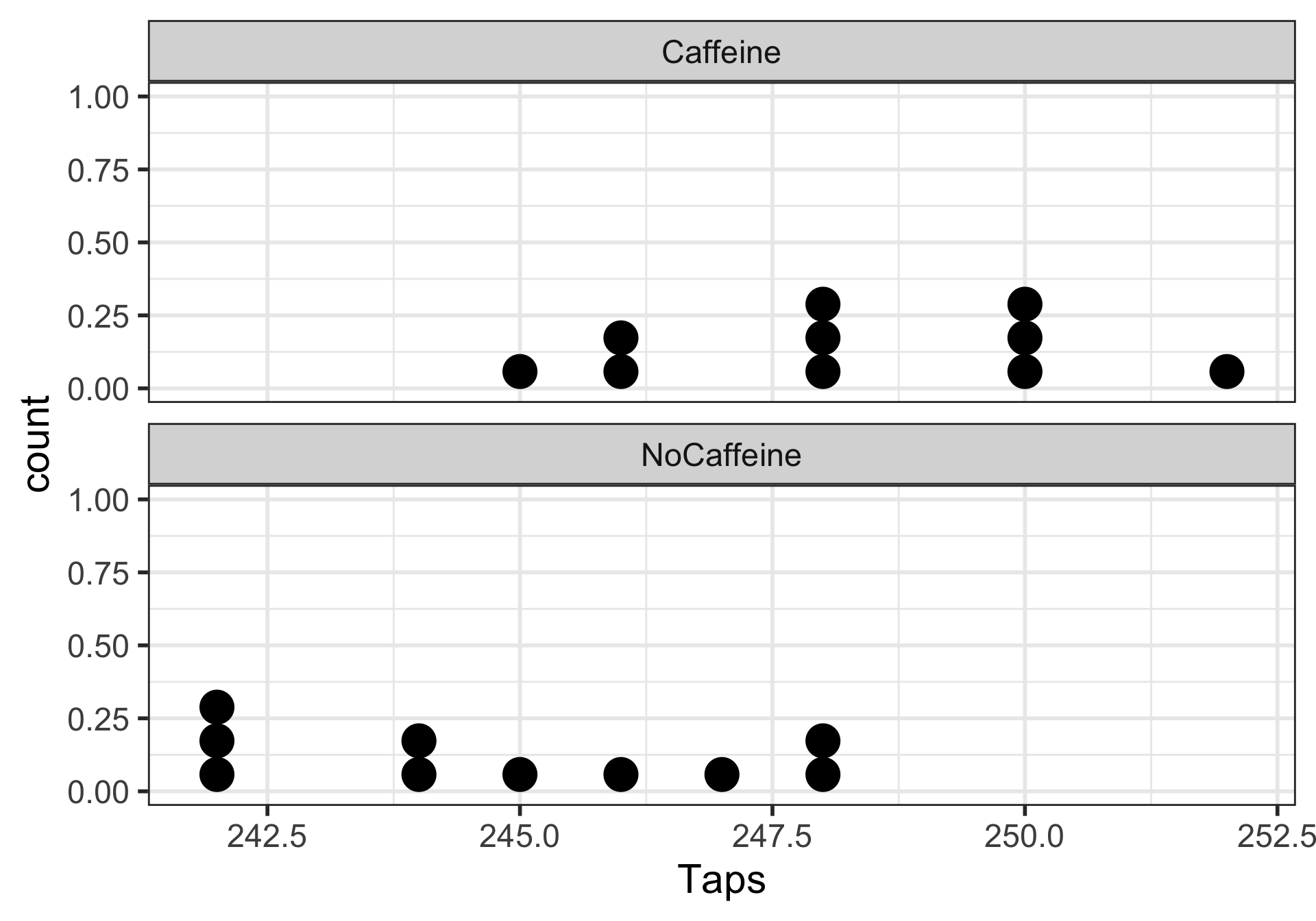
The mean finger taps/min were 244.8 (SD = 2.4) and 248.3 (SD = 2.2) for the control and caffeine groups, and the increase of 3.5 taps/min was statistically discrenible ( \(p\)-value = 0.004).
95% CI for the mean difference in cholesterol levels
Interpretation:
We are 95% confident that the (population) difference in mean finger taps/min between the caffeine and control groups is between 1.167 mg/dL and 5.833 mg/dL.
Based on the CI, is there evidence that drinking caffeine made a difference in finger taps/min? Why or why not?
R: 2-sample t-test (with long data)
The CaffTaps data are in a long format, meaning that
all of the outcome values are in one column and
another column indicates which group the values are from
This is a common format for data from multiple samples, especially if the sample sizes are different.
(Taps_2ttest <-t.test(formula = Taps ~ Group, alternative ="greater", data = CaffTaps))
    Welch Two Sample t-test

data:  Taps by Group
t = 3.3942, df = 17.89, p-value = 0.001628
alternative hypothesis: true difference in means between group Caffeine and group NoCaffeine is greater than 0
95 percent confidence interval:
 1.711272      Inf
sample estimates:
  mean in group Caffeine mean in group NoCaffeine
                   248.3                    244.8
tidy the t.test output
# use tidy command from broom package for briefer output that's a tibbletidy(Taps_2ttest) %>%gt()
estimate
estimate1
estimate2
statistic
p.value
parameter
conf.low
conf.high
method
alternative
3.5
248.3
244.8
3.394168
0.001627703
17.89012
1.711272
Inf
Welch Two Sample t-test
greater
Pull the p-value:
tidy(Taps_2ttest)$p.value # we can pull specific values from the tidy output
[1] 0.001627703
R: 2-sample t-test (with wide data)
# make CaffTaps data wide: pivot_wider needs an ID column so that it # knows how to "match" values from the Caffeine and NoCaffeine groupsCaffTaps_wide <- CaffTaps %>%mutate(id =rep(1:10, 2)) %>%# "fake" IDs for pivot_wider steppivot_wider(names_from ="Group",values_from ="Taps")glimpse(CaffTaps_wide)
The \(t\) distribution degrees of freedom are now:
\[df = (n_1 - 1) + (n_2 - 1) = n_1 + n_2 - 2.\]
R: 2-sample t-test with pooled SD
# t-test with pooled SDt.test(formula = Taps ~ Group, alternative ="greater", var.equal =TRUE, # pooled SD data = CaffTaps) %>%tidy() %>%gt()
estimate
estimate1
estimate2
statistic
p.value
parameter
conf.low
conf.high
method
alternative
3.5
248.3
244.8
3.394168
0.001616497
18
1.711867
Inf
Two Sample t-test
greater
# t-test without pooled SDt.test(formula = Taps ~ Group, alternative ="greater", var.equal =FALSE, # default, NOT pooled SD data = CaffTaps) %>%tidy() %>%gt()
estimate
estimate1
estimate2
statistic
p.value
parameter
conf.low
conf.high
method
alternative
3.5
248.3
244.8
3.394168
0.001627703
17.89012
1.711272
Inf
Welch Two Sample t-test
greater
Similar output in this case - why??
What’s next?
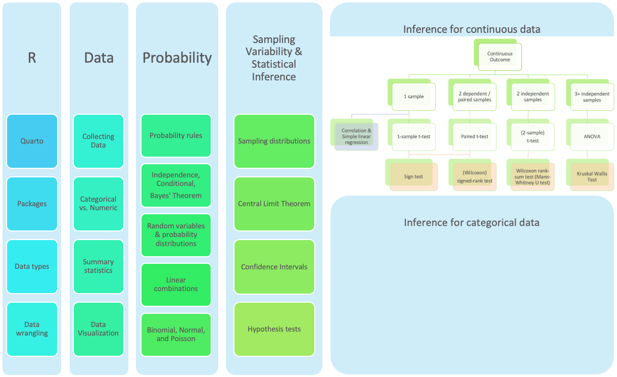
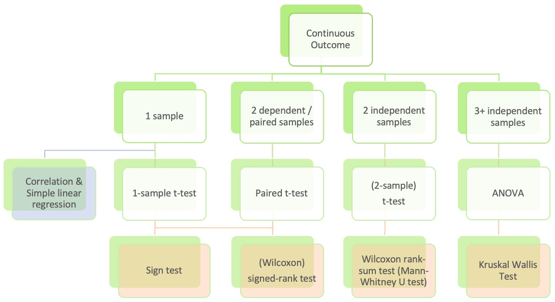
CI’s and hypothesis tests for different scenarios:
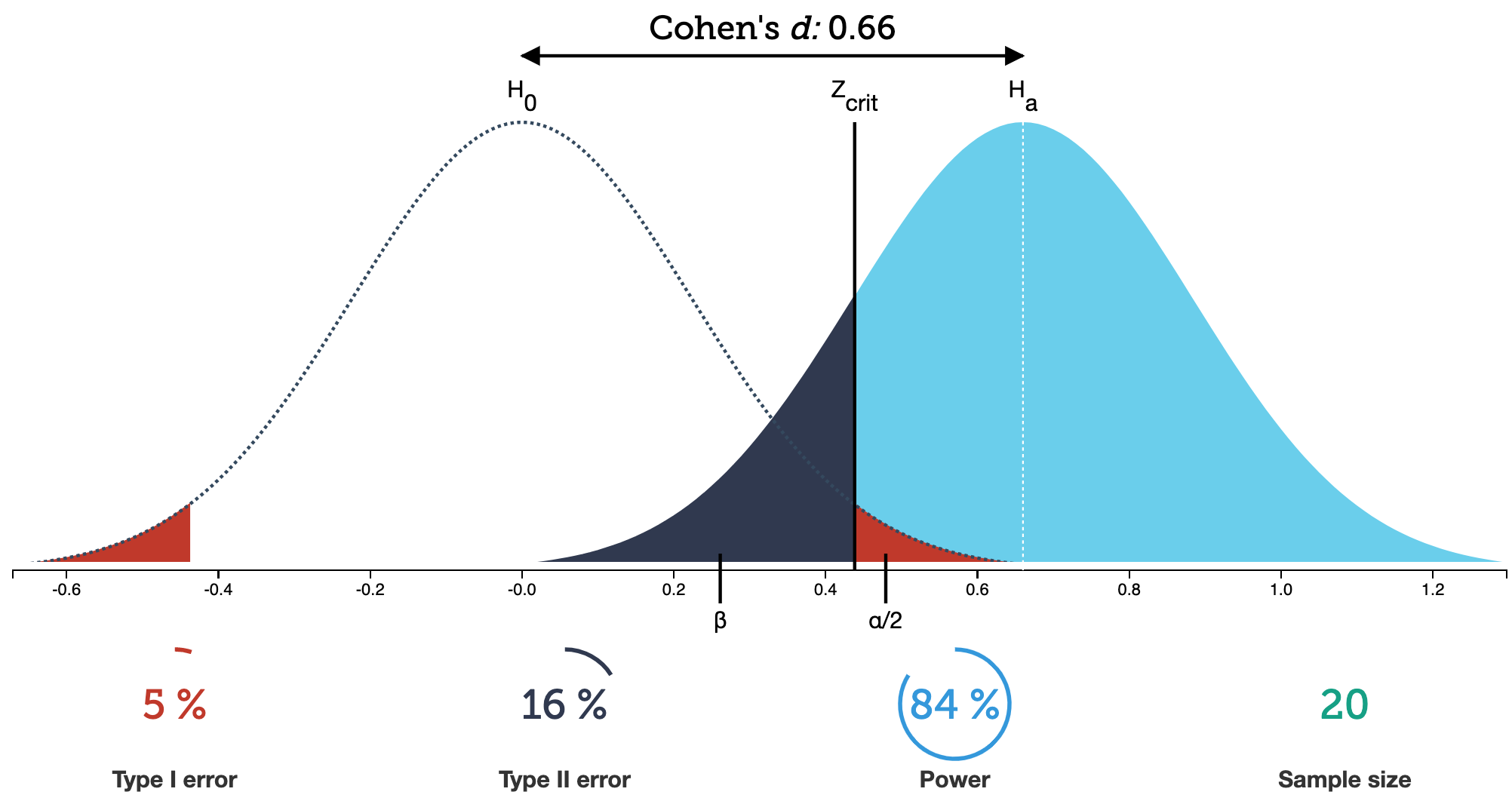
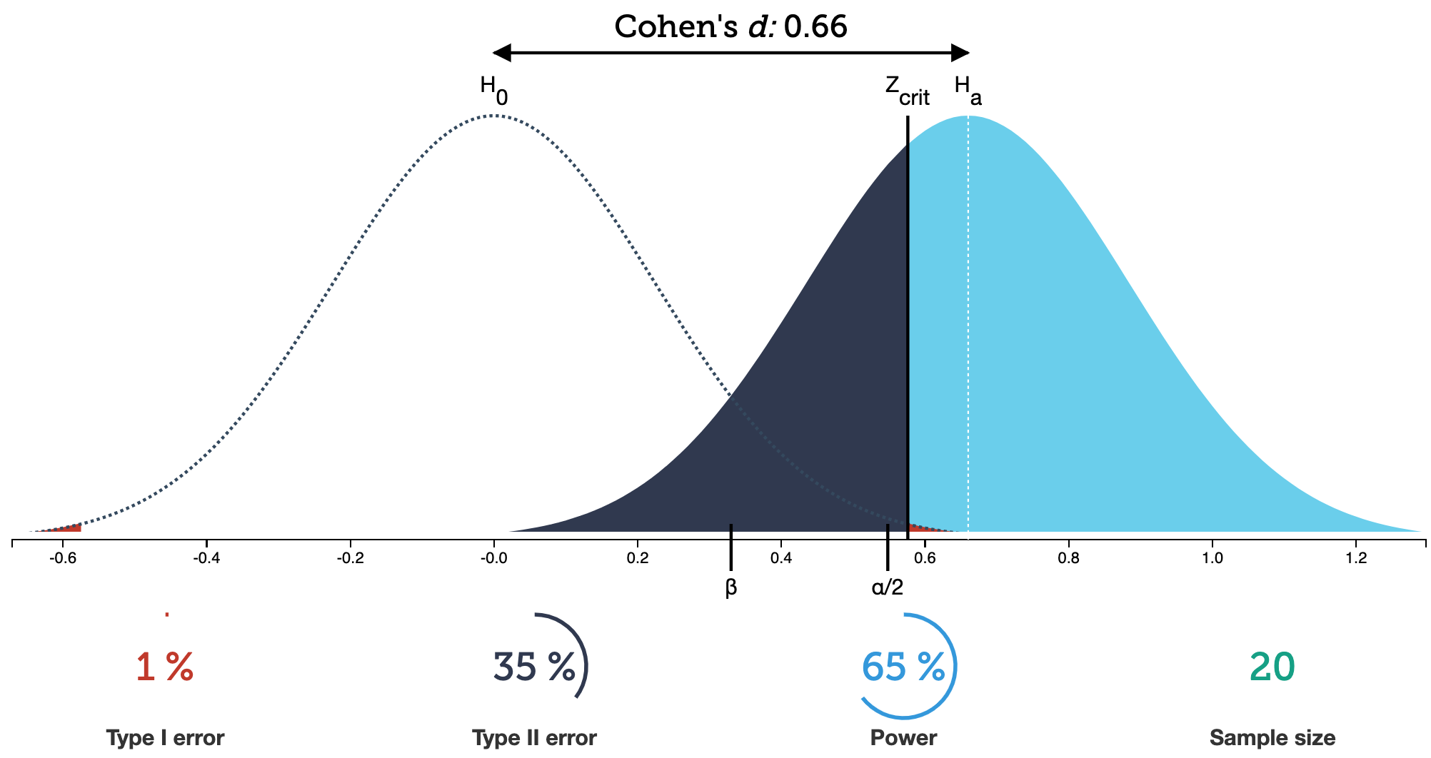
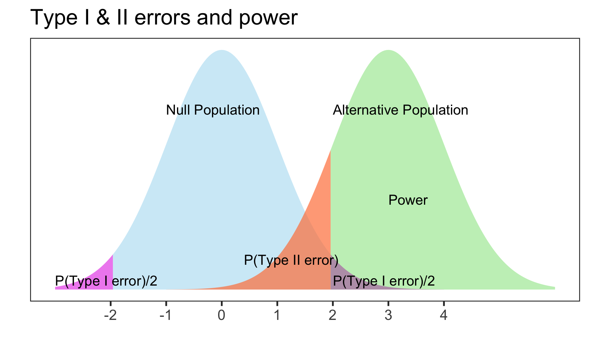
Power = P(correctly rejecting the null hypothesis)
Power is also called the
true positive rate,
probability of detection, or
the sensitivity of a test
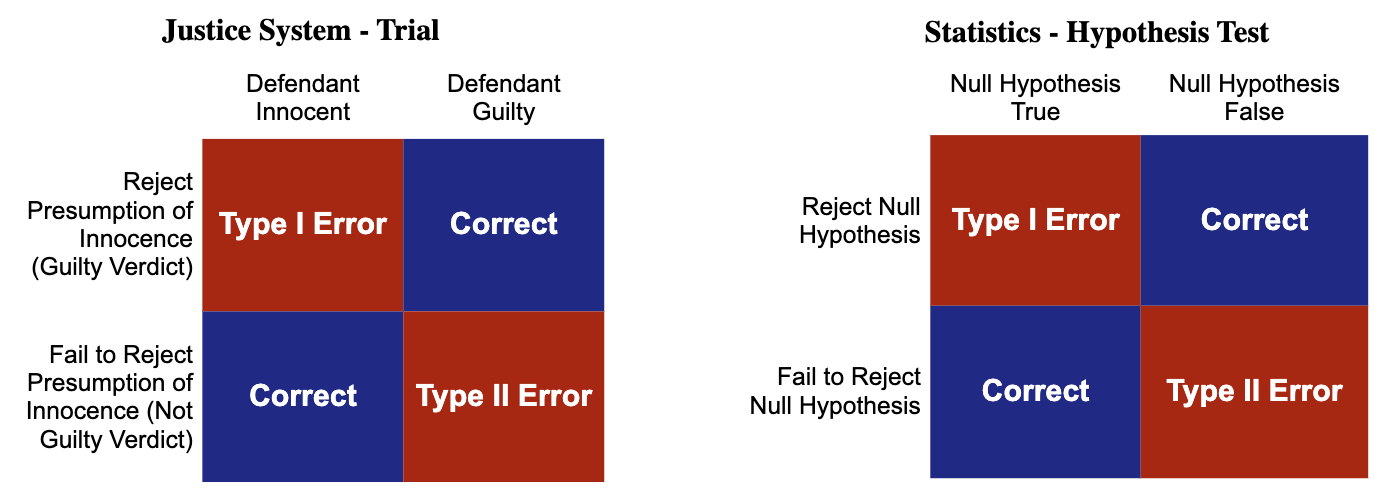
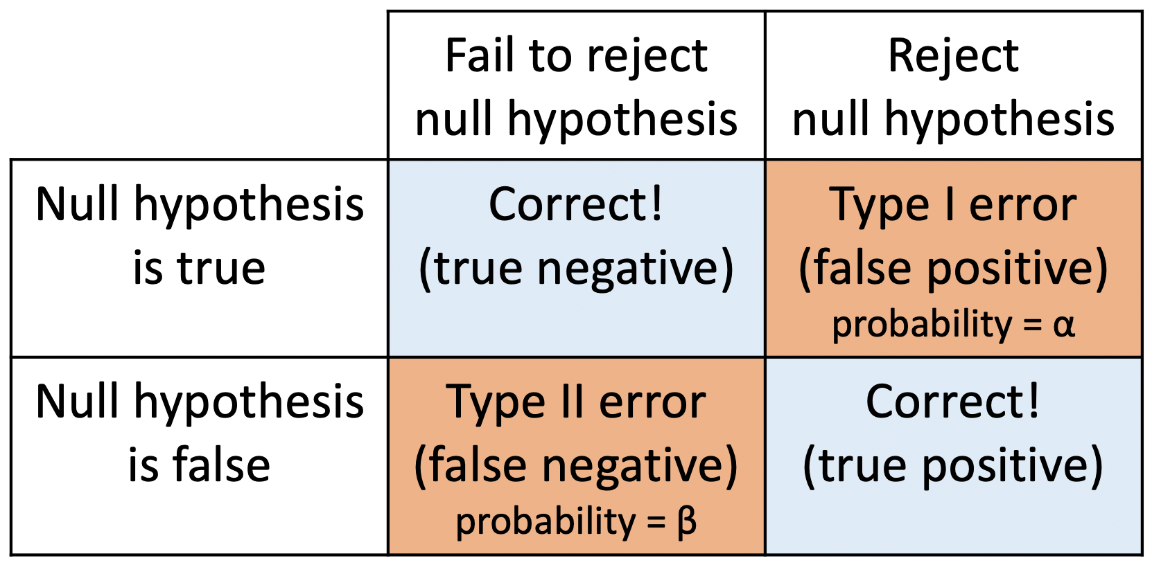
Power vs. Type II error
Power = 1 - P(Type II error) = 1 - \(\beta\)
Thus as \(\beta\) = P(Type II error) decreases, the power increases
P(Type II error) decreases as the mean of the alternative population shifts further away from the mean of the null population (effect size gets bigger).
Typically want at least 80% power; 90% power is good
Example calculating power
Suppose the mean of the null population is 0 ( \(H_0: \mu=0\) ) with standard error 1
Find the power of a 2-sided test if the actual \(\mu=3\), assuming the SE doesn’t change.
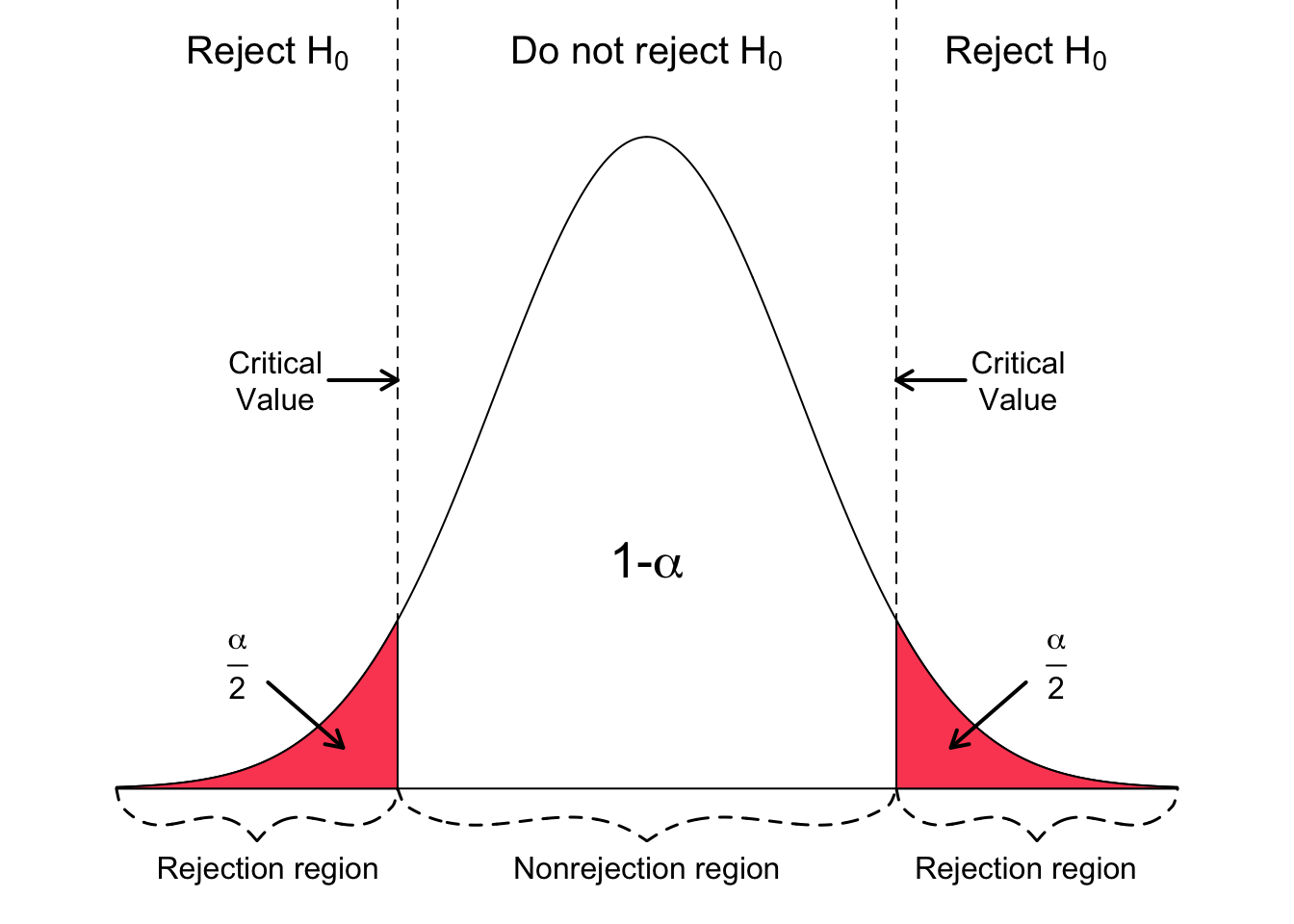
Power = \(P(\)Reject \(H_0\) when alternative pop is \(N(3,1))\)
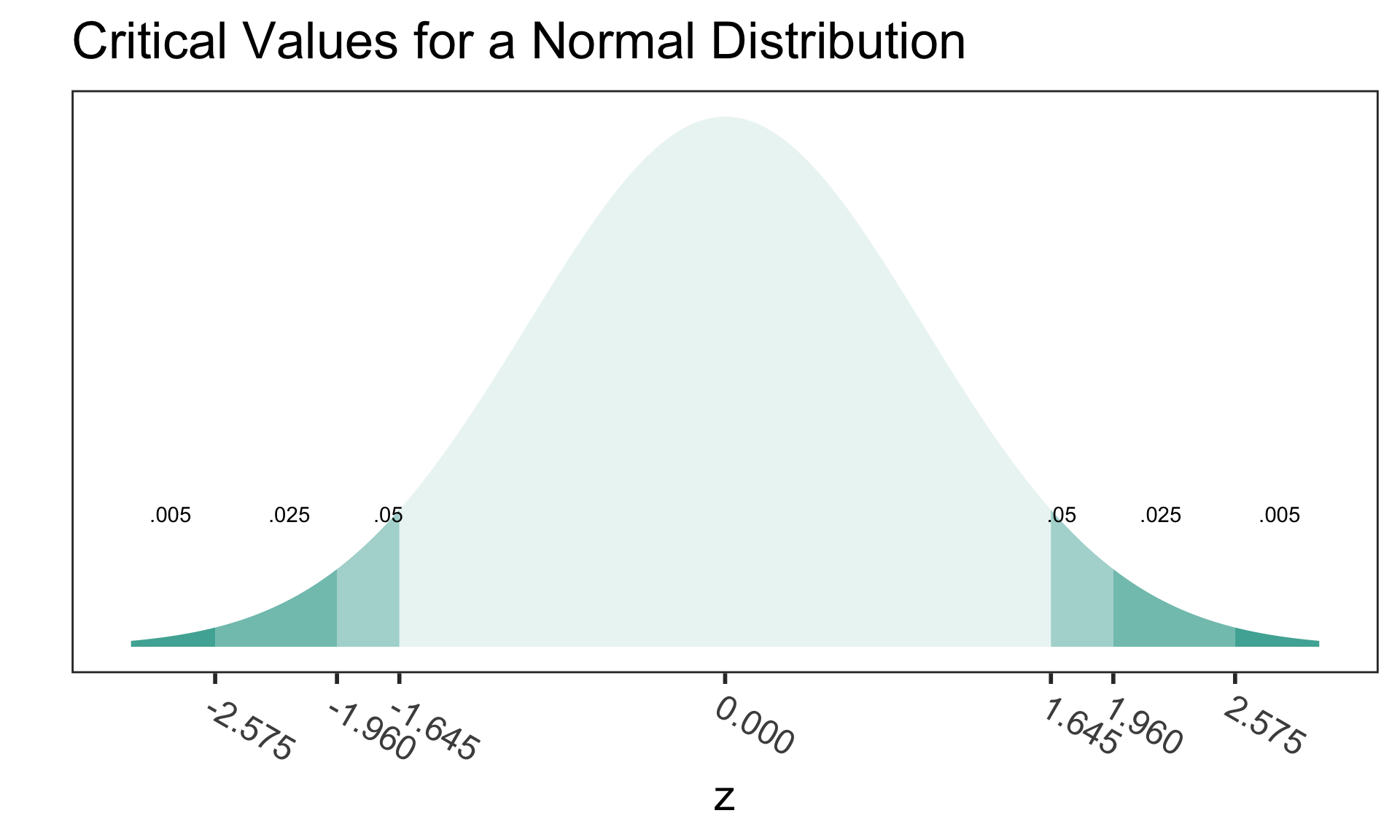
When \(\alpha\) = 0.05, we reject \(H_0\) when the test statistic z is at least 1.96
Thus for \(X\sim N(3,1)\) we need to calculate \(P(X \le -1.96) + P(X \ge 1.96)\):
# left tail + right tail:pnorm(-1.96, mean=3, sd=1, lower.tail=TRUE) +pnorm(1.96, mean=3, sd=1, lower.tail=FALSE)
[1] 0.8508304
The left tail probability pnorm(-1.96, mean=3, sd=1, lower.tail=TRUE) is essentially 0 in this case.
Note that this power calculation specified the value of the SE instead of the standard deviation and sample size \(n\) individually.
Sample size calculation for testing one mean
Recall in our body temperature example that \(\mu_0=98.6\) °F and \(\bar{x}= 98.25\) °F.
The p-value from the hypothesis test was highly significant (very small).
What would the sample size \(n\) need to be for 80% power?
Calculate \(n\),
given \(\alpha\), power ( \(1-\beta\) ), “true” alternative mean \(\mu\), and null \(\mu_0\),
assuming the test statistic is normal (instead of t-distribution):
pwr.t.test(n = NULL, d = NULL, sig.level = 0.05, power = NULL, type = c("two.sample", "one.sample", "paired"),alternative = c("two.sided", "less", "greater"))
d is Cohen’s d effect size: \(d = \frac{\mu-\mu_0}{s}\)
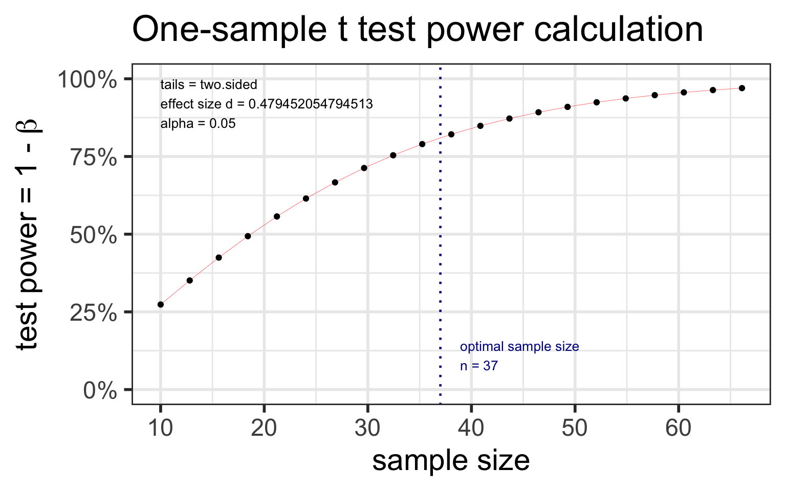
Specify all parameters except for the sample size:
library(pwr)t.n <-pwr.t.test(d = (98.6-98.25)/0.73, sig.level =0.05, power =0.80, type ="one.sample")t.n
     One-sample t test power calculation

              n = 36.11196
              d = 0.4794521
      sig.level = 0.05
          power = 0.8
    alternative = two.sided
plot(t.n)
pwr: power for one mean test
pwr.t.test(n = NULL, d = NULL, sig.level = 0.05, power = NULL, type = c("two.sample", "one.sample", "paired"),alternative = c("two.sided", "less", "greater"))
d is Cohen’s d effect size: \(d = \frac{\mu-\mu_0}{s}\)
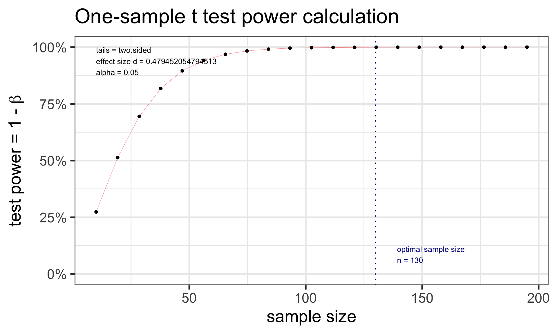
Specify all parameters except for the power:
t.power <-pwr.t.test(d = (98.6-98.25)/0.73, sig.level =0.05, # power = 0.80, n =130,type ="one.sample")t.power
     One-sample t test power calculation

              n = 130
              d = 0.4794521
      sig.level = 0.05
          power = 0.9997354
    alternative = two.sided
plot(t.power)
pwr: Two-sample t-test: sample size
pwr.t.test(n = NULL, d = NULL, sig.level = 0.05, power = NULL, type = c("two.sample", "one.sample", "paired"),alternative = c("two.sided", "less", "greater"))
d is Cohen’s d effect size: \(d = \frac{\bar{x}_1 - \bar{x}_2}{s_{pooled}}\)
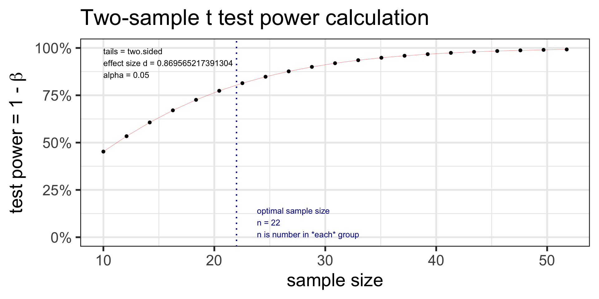
Example: Suppose the data collected for the caffeine taps study were pilot day for a larger study. Investigators want to know what sample size they would need to detect a 2 point difference between the two groups. Assume the SD in both groups is 2.3.
Specify all parameters except for the sample size:
t2.n <-pwr.t.test(d =2/2.3, sig.level =0.05, power =0.80, type ="two.sample") t2.n
     Two-sample t test power calculation

              n = 21.76365
              d = 0.8695652
      sig.level = 0.05
          power = 0.8
    alternative = two.sided

NOTE: n is number in *each* group
plot(t2.n)
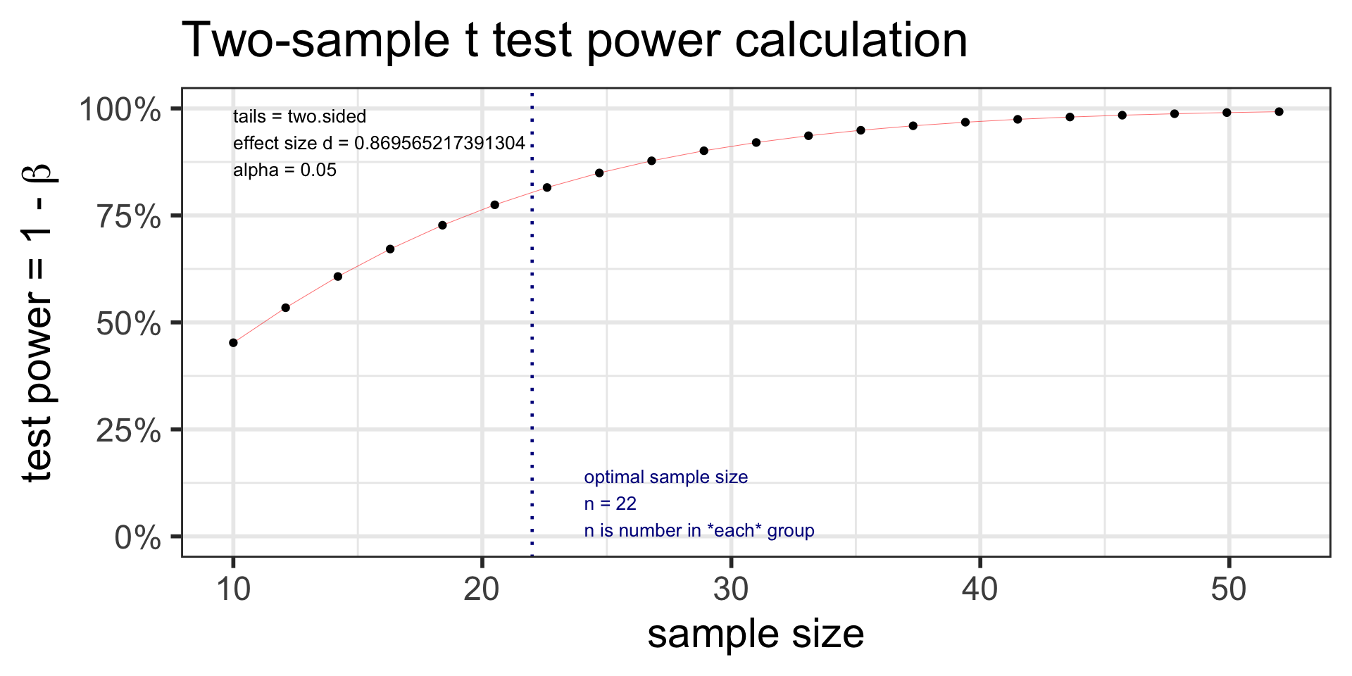
pwr: Two-sample t-test: power
pwr.t.test(n = NULL, d = NULL, sig.level = 0.05, power = NULL, type = c("two.sample", "one.sample", "paired"),alternative = c("two.sided", "less", "greater"))
d is Cohen’s d effect size: \(d = \frac{\bar{x}_1 - \bar{x}_2}{s_{pooled}}\)
Example: Suppose the data collected for the caffeine taps study were pilot day for a larger study. Investigators want to know what sample size they would need to detect a 2 point difference between the two groups. Assume the SD in both groups is 2.3.
Specify all parameters except for the power:
t2.power <-pwr.t.test(d =2/2.3, sig.level =0.05, # power = 0.80, n =22,type ="two.sample") t2.power
     Two-sample t test power calculation

              n = 22
              d = 0.8695652
      sig.level = 0.05
          power = 0.8044288
    alternative = two.sided

NOTE: n is number in *each* group
plot(t2.power)
What information do we need for a power (or sample size) calculation?
There are 4 pieces of information:
Level of significance \(\alpha\)
Usually fixed to 0.05
Power
Ideally at least 0.80
Sample size
Effect size (expected change)
Given any 3 pieces of information, we can solve for the 4th.
pwr.t.test(d = (98.6-98.25)/0.73,sig.level =0.05, # power = 0.80, n=130,type ="one.sample")
     One-sample t test power calculation

              n = 130
              d = 0.4794521
      sig.level = 0.05
          power = 0.9997354
    alternative = two.sided
More software for power and sample size calculations: PASS
PASS is a very powerful (& expensive) software that does power and sample size calculations for many advanced statistical modeling techniques.
Even if you don’t have access to PASS, their documentation is very good and free online.