Day 10 Part 2: Inference for mean difference from two-sample dependent/paired data (Section 5.2)
BSTA 511/611
Week 6
Author
Affiliation
Meike Niederhausen, PhD
OHSU-PSU School of Public Health
Published
November 6, 2024
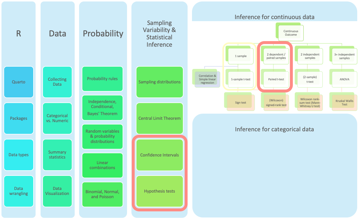
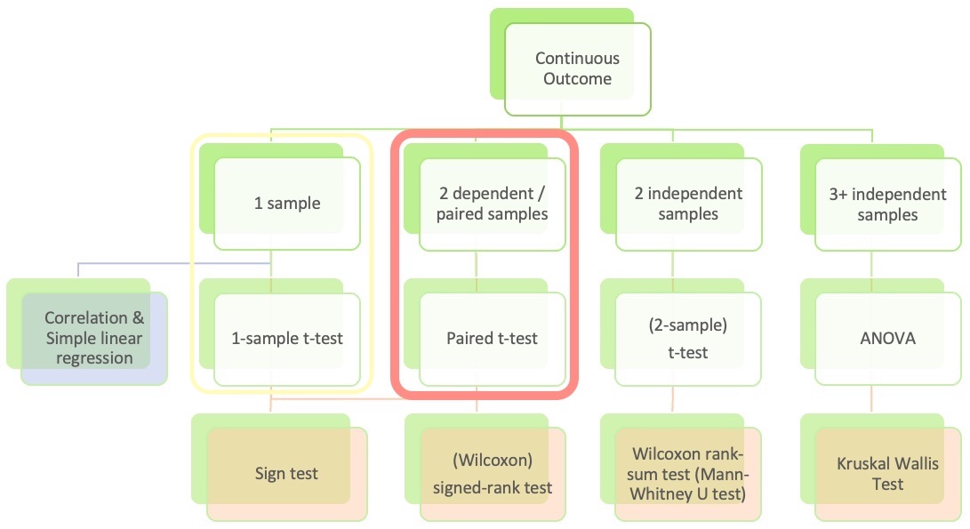
Where are we?
Where are we? Continuous outcome zoomed in
What we covered in Day 10 Part 1
(4.3, 5.1) Hypothesis testing for mean from one sample
Introduce hypothesis testing using the case of analyzing a mean from one sample (group)
Steps of a hypothesis test:
level of significance
null ( \(H_0\) ) and alternative ( \(H_A\) ) hypotheses
test statistic
p-value
conclusion
Run a hypothesis test in R
Load a dataset - need to specify location of dataset
R projects
Run a t-test in R
tidy() the test output using broom package
(4.3.3) Confidence intervals (CIs) vs. hypothesis tests
Goals for today: Part 2 - Class discussion
(5.2) Inference for mean difference from dependent/paired 2 samples
Inference: CIs and hypothesis testing
Exploratory data analysis (EDA) to visualize data
Run paired t-test in R
One-sided CIs
Class discussion
Inference for the mean difference from dependent/paired data is a special case of the inference for the mean from just one sample, that was already covered.
Thus this part will be used for class discussion to practice CIs and hypothesis testing for one mean and apply it in this new setting.
In class I will briefly introduce this topic, explain how it is similar and different from what we already covered, and let you work through the slides and code.
CI’s and hypothesis tests for different scenarios:
Rows: 24 Columns: 2
── Column specification ────────────────────────────────────────────────────────
Delimiter: ","
dbl (2): Before, After

ℹ Use `spec()` to retrieve the full column specification for this data.
ℹ Specify the column types or set `show_col_types = FALSE` to quiet this message.
Based on the value of the test statistic, do you think we are going to reject or fail to reject \(H_0\)?
What probability distribution does the test statistic have?
Are the assumptions for a paired t-test satisfied so that we can use the probability distribution to calculate the \(p\)-value??
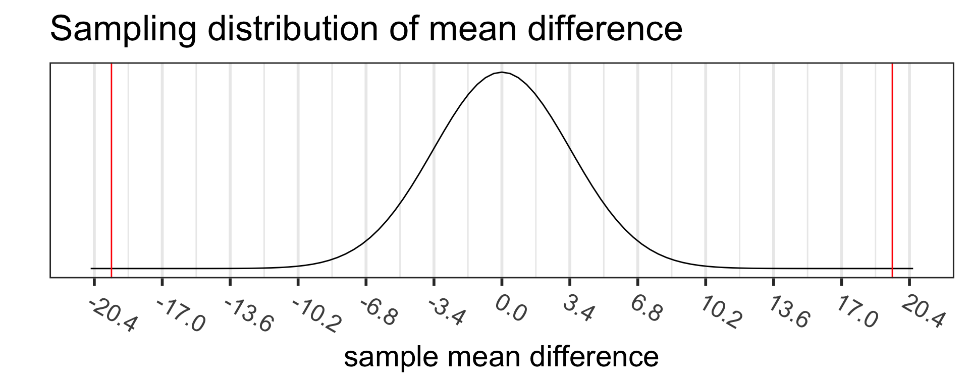
Step 4: p-value
The p-value is the probability of obtaining a test statistic just as extreme or more extreme than the observed test statistic assuming the null hypothesis \(H_0\) is true.
Calculate the p-value and shade in the area representing the p-value:
Recall the \(p\)-value = \(8.434775 \cdot 10 ^{-6}\)
Use \(\alpha\) = 0.05.
Do we reject or fail to reject \(H_0\)?
Conclusion statement:
Stats class conclusion
There is sufficient evidence that the (population) mean difference in cholesterol levels after a vegetarian diet is different from 0 mg/dL ( \(p\)-value < 0.001).
More realistic manuscript conclusion:
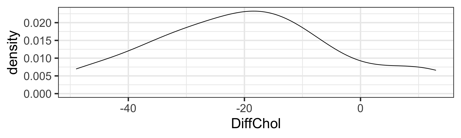
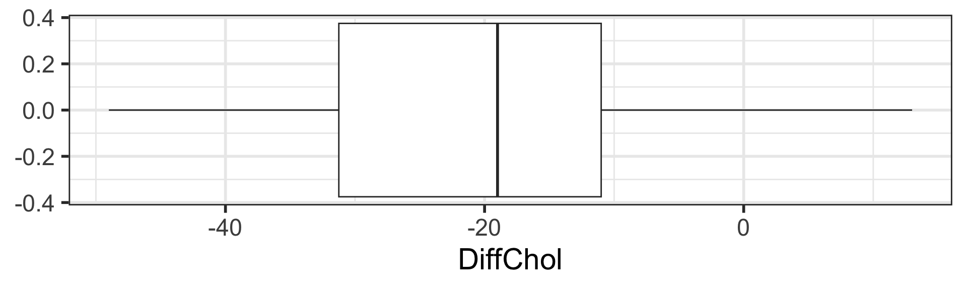
After a vegetarian diet, cholesterol levels decreased by on average 19.54 mg/dL (SE = 3.43 mg/dL, 2-sided \(p\)-value < 0.001).
95% CI for the mean difference in cholesterol levels
Conclusion:
We are 95% that the (population) mean difference in cholesterol levels after a vegetarian diet is between -26.638 mg/dL and -12.445 mg/dL.
Based on the CI, is there evidence the diet made a difference in cholesterol levels? Why or why not?
Running a paired t-test in R
R option 1: Run a 1-sample t.test using the paired differences
\(H_A: \delta \neq 0\)
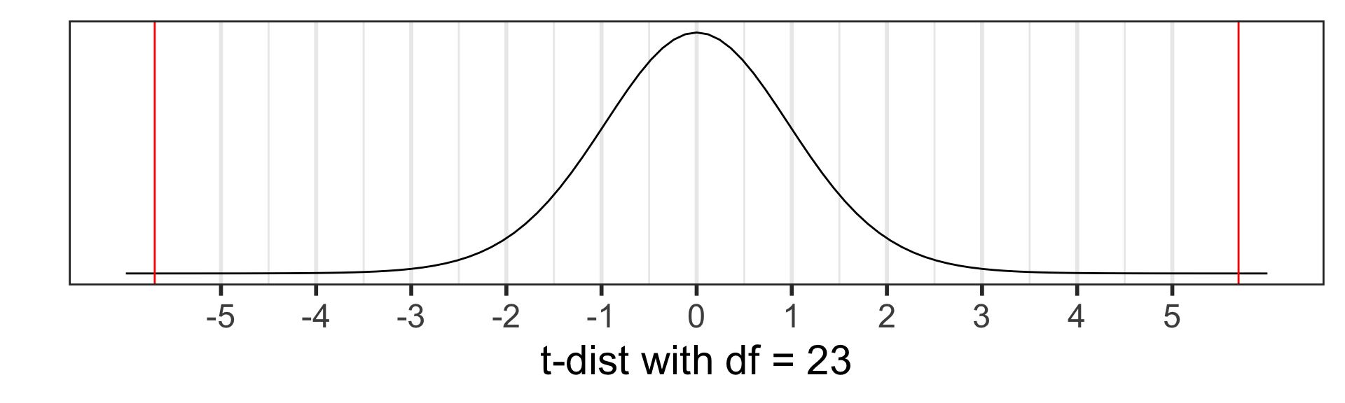
t.test(x = chol$DiffChol, mu =0)
    One Sample t-test

data:  chol$DiffChol
t = -5.6965, df = 23, p-value = 8.435e-06
alternative hypothesis: true mean is not equal to 0
95 percent confidence interval:
 -26.63811 -12.44522
sample estimates:
mean of x
-19.54167
Run the code without mu = 0. Do the results change? Why or why not?
R option 2: Run a 2-sample t.test with paired = TRUE option
\(H_A: \delta \neq 0\)
For a 2-sample t-test we specify both x= and y=
Note: mu = 0 is the default value and doesn’t need to be specified
t.test(x = chol$Before, y = chol$After, mu =0, paired =TRUE)
    Paired t-test

data:  chol$Before and chol$After
t = 5.6965, df = 23, p-value = 8.435e-06
alternative hypothesis: true mean difference is not equal to 0
95 percent confidence interval:
 12.44522 26.63811
sample estimates:
mean difference
       19.54167
What is different in the output compared to option 1?
R option 3: Run a 2-sample t.test with paired = TRUE option, but using the long data and a “formula” (1/2)
The data have to be in a long format for option 3, where each person has 2 rows: one for Before and one for After.
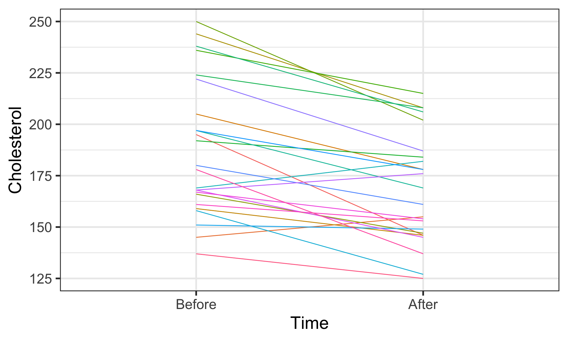
The long dataset chol_long was created for the slide “EDA: Spaghetti plot of cholesterol levels before & after diet”.
See the code to create it there.
What information is being stored in each of the columns?
# first 16 rows of long data:head(chol_long, 16)
# A tibble: 16 × 3
   ID    Time   Cholesterol
   <fct> <fct>        <dbl>
 1 1     Before         195
 2 1     After          146
 3 2     Before         145
 4 2     After          155
 5 3     Before         205
 6 3     After          178
 7 4     Before         159
 8 4     After          146
 9 5     Before         244
10 5     After          208
11 6     Before         166
12 6     After          147
13 7     Before         250
14 7     After          202
15 8     Before         236
16 8     After          215
R option 3: Run a 2-sample t.test with paired = TRUE option, but using the long data and a “formula” (2/2)
Use the usual t.test
What’s different is that
instead of specifying the variables with x= and y=,
we give a formula of the form y ~ x using just the variable names,
and then specify the name of the dataset using data =
This method is often used in practice, and more similar to the coding style of running a regression model (BSTA 512 & 513)
# using long data # with columns Cholesterol & Timet.test(Cholesterol ~ Time, paired =TRUE, data = chol_long)
    Paired t-test

data:  Cholesterol by Time
t = 5.6965, df = 23, p-value = 8.435e-06
alternative hypothesis: true mean difference is not equal to 0
95 percent confidence interval:
 12.44522 26.63811
sample estimates:
mean difference
       19.54167
What is different in the output compared to option 1?
Rerun the test using Time ~ Cholesterol (switch the variables). What do you get?
Compare the 3 options
How is the code similar and different for the 3 options?
Given a dataset, how would you choose which of the 3 options to use?
# option 1t.test(x = chol$DiffChol, mu =0) %>%tidy() %>%gt() # tidy from broom package
estimate
statistic
p.value
parameter
conf.low
conf.high
method
alternative
-19.54167
-5.696519
8.434775e-06
23
-26.63811
-12.44522
One Sample t-test
two.sided
# option 2t.test(x = chol$Before, y = chol$After, mu =0, paired =TRUE) %>%tidy() %>%gt()
estimate
statistic
p.value
parameter
conf.low
conf.high
method
alternative
19.54167
5.696519
8.434775e-06
23
12.44522
26.63811
Paired t-test
two.sided
# option 3t.test(Cholesterol ~ Time, paired =TRUE, data = chol_long) %>%tidy() %>%gt()
estimate
statistic
p.value
parameter
conf.low
conf.high
method
alternative
19.54167
5.696519
8.434775e-06
23
12.44522
26.63811
Paired t-test
two.sided
What if we wanted to test whether the diet decreased cholesterol levels?
What changes in each of the steps?
Set the level of significance\(\alpha\)
Specify the hypotheses\(H_0\) and \(H_A\)
Alternative: one- or two-sided?
Calculate the test statistic.
Calculate the p-value based on the observed test statistic and its sampling distribution
Write a conclusion to the hypothesis test
R: What if we wanted to test whether the diet decreased cholesterol levels?
Which of the 3 options to run a paired t-test in R is being used below?
How did the code change to account for testing a decrease in cholesterol levels?
Which values in the output changed compared to testing for a change in cholesterol levels? How did they change?
# alternative = c("two.sided", "less", "greater")t.test(x = chol$DiffChol, mu =0, alternative ="less") %>%tidy() %>%gt()
estimate
statistic
p.value
parameter
conf.low
conf.high
method
alternative
-19.54167
-5.696519
4.217387e-06
23
-Inf
-13.6623
One Sample t-test
less
One-sided confidence intervals
Formula for a 2-sided (1- \(\alpha\) )% CI:
\[\bar{x} \pm t^*\cdot\frac{s}{\sqrt{n}}\]
\(t^*\) = qt(1-alpha/2, df = n-1)
\(\alpha\) is split over both tails of the distribution
A one-sided (1- \(\alpha\) )% CI has all (1- \(\alpha\) )% on just the left or the right tail of the distribution: