Day 2: Data collection & numerical summaries

BSTA 511/611 Fall 2024 Days 2-4, OHSU

Goals for today

• (1.3) Data collection principles - Day 2 in F24
  • Population vs. sample
  • Sampling methods
  • Experiments vs. Observational studies
• (1.2) Intro to Data - Day 2 in F24
  • Data types
  • How are data stored in R?
  • Working with data in R
• (1.4) Summarizing numerical data - Day 3 in F24
  • Mean, median, mode, SD, IQR, range, 5 number summary
  • Empirical Rule
  • robust statistics
• R packages - Day 4 in F24 -> install for Day 5!!!

Recap of last time

• Open RStudio on your computer (not R!)

Modern Dive

• Basic math using R

• Creating and rendering Quarto files

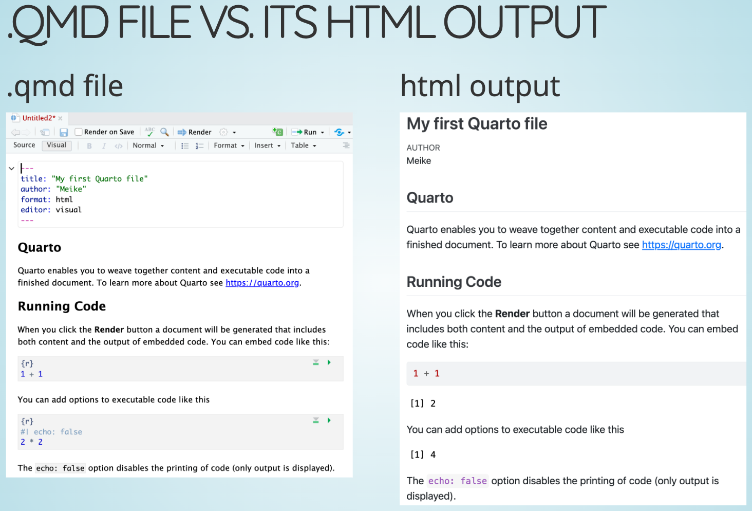
• Formatting text & headers
• Code chunks

Useful keyboard shortcuts

Full list of keyboard shortcuts
 

action	mac	windows/linux
Run code in qmd (or script)	cmd + enter	ctrl + enter
<-	option + -	alt + -
interrupt currently running command	esc	esc
in console, retrieve previously run code	up/down	up/down
keyboard shortcut help	option + shift + k	alt + shift + k

Practice

Try typing code below in your qmd (with shortcut) and evaluating it:

y <- 5
y

Another resource for an introduction to R

• If you would like another perspective on what we covered the first week, you might find Danielle Navarro’s online book Learning Statistics with R to be helpful.

• Download free pdf: https://learningstatisticswithr.com/

• See Sections 3.1-3.7.1 for some of the topics we covered on first day

MoRitz’s tip of the day

Customize your RStudio interface!
https://www.pipinghotdata.com/posts/2020-09-07-introducing-the-rstudio-ide-and-r-markdown/#background

(1.3) Data collection principles - Day 2 in F24

• Population vs. sample
• Sampling methods
• Experiments vs. Observational studies

Population vs. sample

(Target) Population

• group of interest being studied
• group from which the sample is selected
  • studies often have inclusion and/or exclusion criteria

Sample

• group on which data are collected
• often a small subset of the population

Sampling methods (1/4)

Goal is to get a representative sample of the population:
the characteristics of the sample are similar to the characteristics of the population

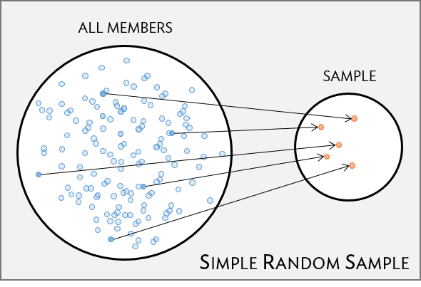
Simple random sample (SRS)

• each individual of a population has the same chance of being sampled
• randomly sampled
• considered best way to sample

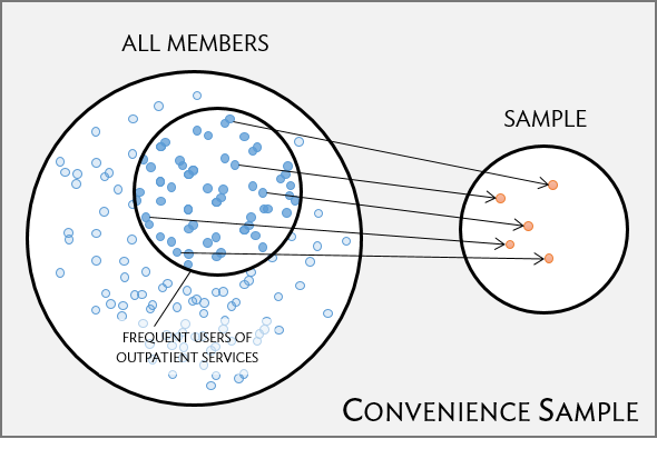
Convenience sample

• easily accessible individuals are more likely to be included in the sample than other individuals
• a common “pitfall”

Sampling methods (2/4)

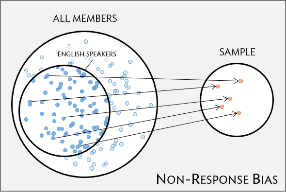
Good sampling plans don’t guarantee samples representative of the population

Non-response bias

• non-response rates can be high
• are all groups within a population being reached?
• unrepresentative sample
  => skewed results

“Random” samples can be unrepresentative by random chance

• In a SRS each case in the population has an equal chance of being included in the sample
• But by random chance alone a random sample might contain a higher proportion of one group over another
• Ex: a SRS might by chance include 70% men (unlikely, but theoretically possible)

Sampling methods (3/4)

• Simple random sample (SRS)
  • each individual of a population has the same chance of being sampled
  • statistical methods taught in this class assume a SRS!
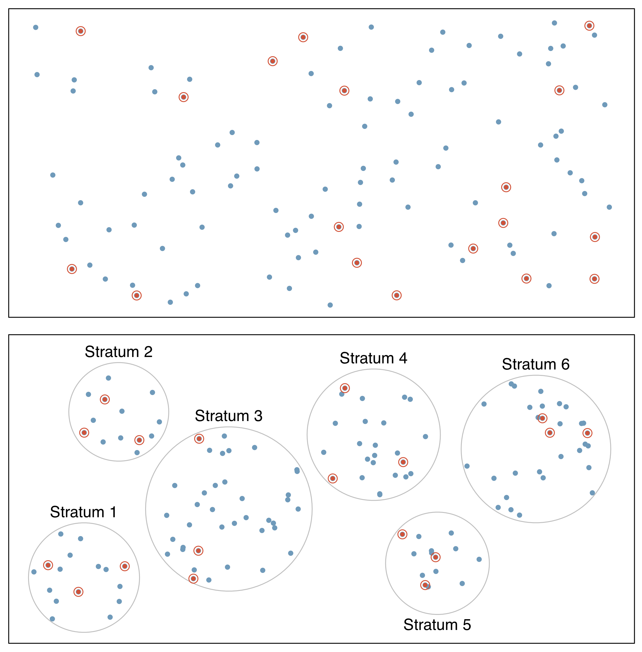
• Stratified sampling
  • divide population into groups (strata) before selecting cases within each stratum (often via SRS)
  • usually cases within a strata are similar, but are different from other strata with respect to the outcome of interest, such as gender or age groups

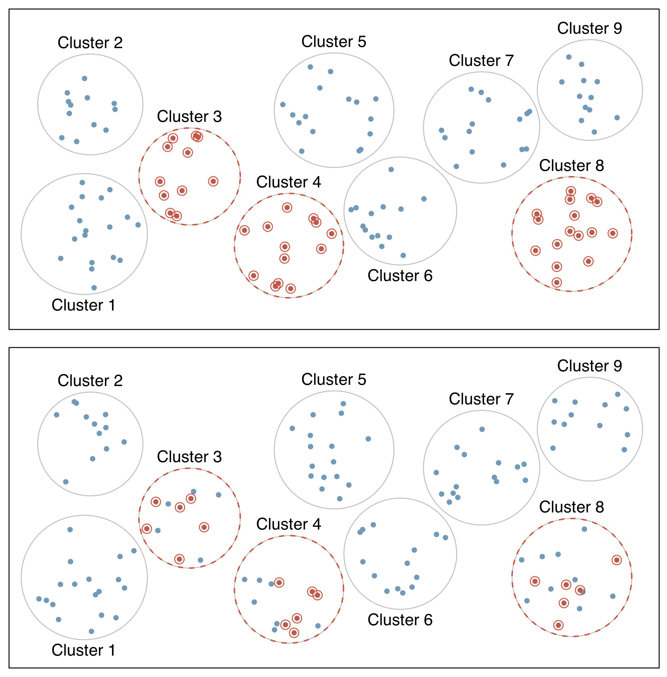
Sampling methods (4/4)

• Cluster sample
  • first divide population into groups (clusters)
  • then sample a fixed number of clusters, and include all observations from chosen clusters
  • clusters are often hospitals, clinicians, schools, etc., where each cluster will have similar services/ policies/ etc.
  • cases within clusters usually very diverse
• Multistage sample
  • similar to a cluster sample, but select a random sample within each selected cluster instead of all individuals

Experiments (1/2)

• Researchers assign individuals to different treatment or intervention groups
  • control group: often receive a placebo or usual care
  • different treatment groups are often called study arms
• Randomization
  • group assignment is usually random to ensure similar (balanced) study arms for all variables (observed and unobserved)
  • randomization allows study arm differences in outcomes to be attributed to treatment rather than variability in patient characteristics
    • treatment is the only systematic difference between groups
    • establish causality
  • blocking (stratification): group individuals into blocks (strata) before randomizing if there are certain characteristics that may influence the outcome other than treatment (i.e. gender, age group)

Experiments (2/2)

• Replication
  • accomplished by collecting a sufficiently large sample
  • results usually more reliable with a large sample size
    • often less variability
    • more likely to be representative of population
• Some studies are not ethical to carry out as experiments

Observational studies

• data are observed and recorded without interference
• often done via surveys, electronic health records, or medical chart reviews
• cohorts
• associations between variables can be established, but not causality
  • Individuals with different characteristics may also differ in other ways that influence response
• confounding variables (lurking variable)
  • variables associated with both the explanatory and response variables
• prospective vs. retrospective studies

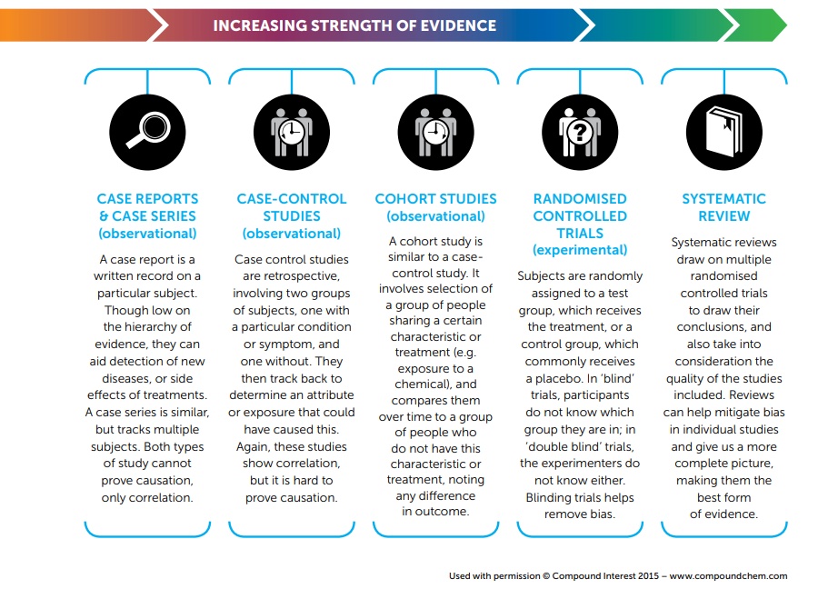
Comparing study designs

Science Media Centre

Systematic Reviews example

STEM: Systematically Testing the Evidence on Marijuana

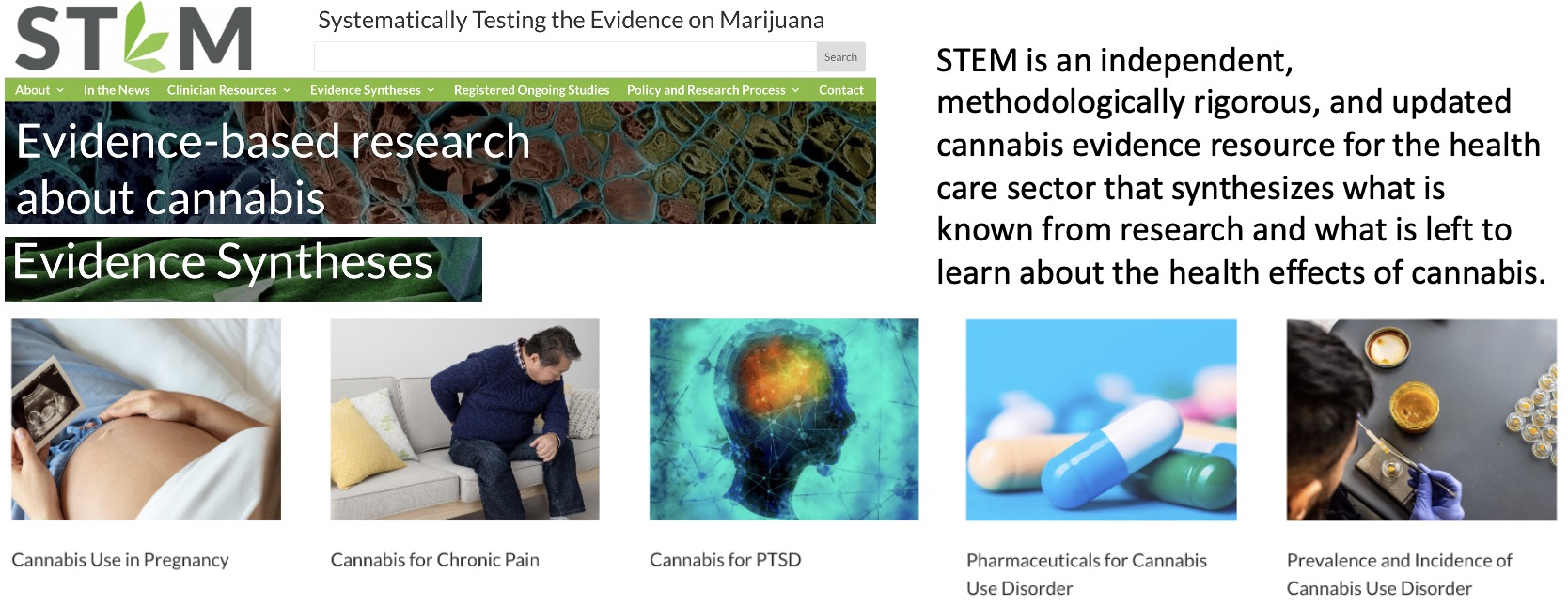
STEM is a collaborative project between the US Department of Veterans Affairs and the Center for Evidence-based Policy at Oregon Health & Science University.
The project is funded by the US Department of Veterans Affairs: Office of Rural Health.

(1.2) Intro to Data - Day 2 in F24

Artwork by @allison_horst

How are data stored, how do we use them?

• Often, data are in an Excel sheet, or a plain text file (.csv, .txt)
• .csv files open in Excel automatically, but actually are plain text
• Usually, columns are variables/measures and rows are observations (i.e. a person’s measurements)

Data in R

• We can import data from many file types, including .csv, .txt., and .xlsx
  • We will cover this on a later date
• Once imported, R typically stores data as data frames, or tibbles if using the tidyverse package (more on this later).
  • For our purposes, these are essentially the same, and I will tend to use the terms interchangeably.
  • These are examples of what we call object types in R.

Data frame example

df <- data.frame(
  IDs=1:3, 
  gender=c("male", "female", "Male"), 
  age=c(28, 35.5, 31),
  trt = c("control", "1", "1"),
  Veteran = c(FALSE, TRUE, TRUE)
  )
df

  IDs gender  age     trt Veteran
1   1   male 28.0 control   FALSE
2   2 female 35.5       1    TRUE
3   3   Male 31.0       1    TRUE

• Vectors vs. data frames
  • a data frame is a collection (or array or table) of vectors

• Different columns can be of different data types (i.e. numeric vs. text)

• Both numeric and text can be stored within a column (stored together as text).

• Vectors and data frames are examples of objects in R.

  • There are other types of R objects to store data, such as matrices, lists.

Observations & variables

df

  IDs gender  age     trt Veteran
1   1   male 28.0 control   FALSE
2   2 female 35.5       1    TRUE
3   3   Male 31.0       1    TRUE

ISLBS

• Book refers to a dataset as a data matrix

• Rows are usually observations

• Columns are usually variables

• How many observations are in this dataset?

• What are the variable types in this dataset?

Variable (column) types

R type	variable type	description
integer	discrete	integer-valued numbers
double or numeric	continuous	numbers that are decimals
factor	categorical	categorical variables stored with levels (groups)
character	categorical	text, “strings”
logical	categorical	boolean (TRUE, FALSE)

• View the structure of our data frame to see what the variable types are:

str(df)

'data.frame':   3 obs. of  5 variables:
 $ IDs    : int  1 2 3
 $ gender : chr  "male" "female" "Male"
 $ age    : num  28 35.5 31
 $ trt    : chr  "control" "1" "1"
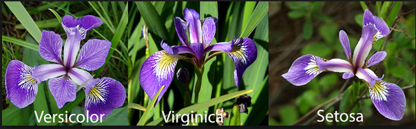
 $ Veteran: logi  FALSE TRUE TRUE

Fisher’s (or Anderson’s) Iris data set

Data description:

• n = 150
• 3 species of Iris flowers (Setosa, Virginica, and Versicolour)
  • 50 measurements of each type of Iris
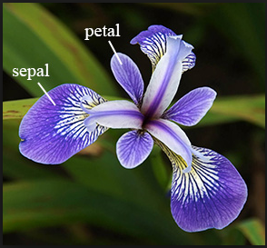
• variables:
  • sepal length, sepal width, petal length, petal width, and species

Can the iris species be determined by these variables?

Gareth Duffy

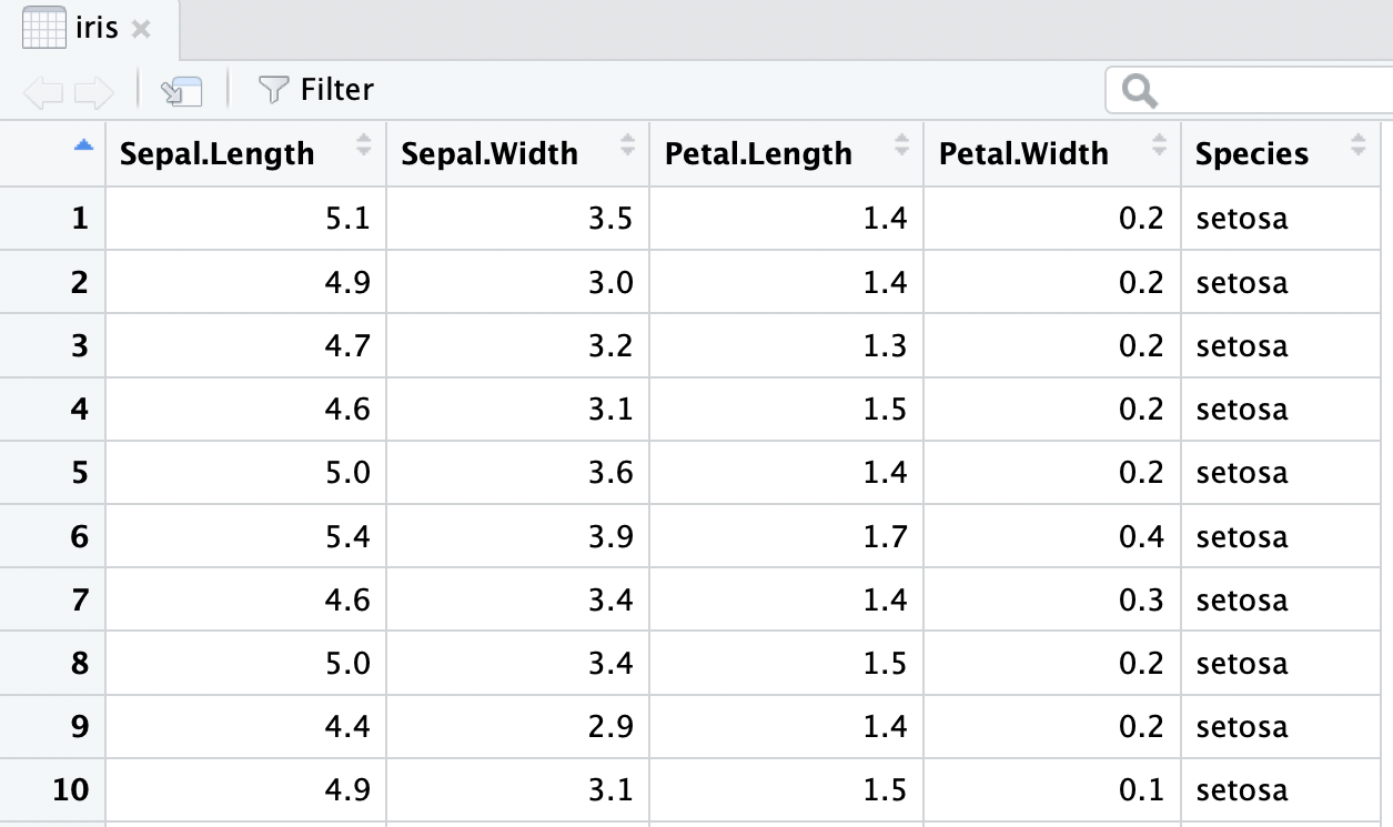
View the iris dataset

• The iris dataset is already pre-loaded in base R and ready to use.
• Type the following command in the console window
  • Warning: this command cannot be rendered. It will give an error.

View(iris)

A new tab in the scripting window should appear with the iris dataset.

Data structure

• What are the different variable types in this data set?

str(iris)   # structure of data

'data.frame':   150 obs. of  5 variables:
 $ Sepal.Length: num  5.1 4.9 4.7 4.6 5 5.4 4.6 5 4.4 4.9 ...
 $ Sepal.Width : num  3.5 3 3.2 3.1 3.6 3.9 3.4 3.4 2.9 3.1 ...
 $ Petal.Length: num  1.4 1.4 1.3 1.5 1.4 1.7 1.4 1.5 1.4 1.5 ...
 $ Petal.Width : num  0.2 0.2 0.2 0.2 0.2 0.4 0.3 0.2 0.2 0.1 ...
 $ Species     : Factor w/ 3 levels "setosa","versicolor",..: 1 1 1 1 1 1 1 1 1 1 ...

Data set summary

summary(iris)

  Sepal.Length    Sepal.Width     Petal.Length    Petal.Width   
 Min.   :4.300   Min.   :2.000   Min.   :1.000   Min.   :0.100  
 1st Qu.:5.100   1st Qu.:2.800   1st Qu.:1.600   1st Qu.:0.300  
 Median :5.800   Median :3.000   Median :4.350   Median :1.300  
 Mean   :5.843   Mean   :3.057   Mean   :3.758   Mean   :1.199  
 3rd Qu.:6.400   3rd Qu.:3.300   3rd Qu.:5.100   3rd Qu.:1.800  
 Max.   :7.900   Max.   :4.400   Max.   :6.900   Max.   :2.500  
       Species  
 setosa    :50  
 versicolor:50  
 virginica :50  
                
                
                

Data set info

dim(iris)

[1] 150   5

nrow(iris)

[1] 150

ncol(iris)

[1] 5

names(iris)

[1] "Sepal.Length" "Sepal.Width"  "Petal.Length" "Petal.Width"  "Species"     

View the beginning or end of a dataset

head(iris)

  Sepal.Length Sepal.Width Petal.Length Petal.Width Species
1          5.1         3.5          1.4         0.2  setosa
2          4.9         3.0          1.4         0.2  setosa
3          4.7         3.2          1.3         0.2  setosa
4          4.6         3.1          1.5         0.2  setosa
5          5.0         3.6          1.4         0.2  setosa
6          5.4         3.9          1.7         0.4  setosa

tail(iris)

    Sepal.Length Sepal.Width Petal.Length Petal.Width   Species
145          6.7         3.3          5.7         2.5 virginica
146          6.7         3.0          5.2         2.3 virginica
147          6.3         2.5          5.0         1.9 virginica
148          6.5         3.0          5.2         2.0 virginica
149          6.2         3.4          5.4         2.3 virginica
150          5.9         3.0          5.1         1.8 virginica

Specify how many rows to view at beginning or end of a dataset

head(iris, 3)

  Sepal.Length Sepal.Width Petal.Length Petal.Width Species
1          5.1         3.5          1.4         0.2  setosa
2          4.9         3.0          1.4         0.2  setosa
3          4.7         3.2          1.3         0.2  setosa

tail(iris, 2)

    Sepal.Length Sepal.Width Petal.Length Petal.Width   Species
149          6.2         3.4          5.4         2.3 virginica
150          5.9         3.0          5.1         1.8 virginica

The $

• Suppose we want to single out the column of petal width values.
• One way to do this is to use the $
  • DatSetName$VariableName

iris$Petal.Width

  [1] 0.2 0.2 0.2 0.2 0.2 0.4 0.3 0.2 0.2 0.1 0.2 0.2 0.1 0.1 0.2 0.4 0.4 0.3
 [19] 0.3 0.3 0.2 0.4 0.2 0.5 0.2 0.2 0.4 0.2 0.2 0.2 0.2 0.4 0.1 0.2 0.2 0.2
 [37] 0.2 0.1 0.2 0.2 0.3 0.3 0.2 0.6 0.4 0.3 0.2 0.2 0.2 0.2 1.4 1.5 1.5 1.3
 [55] 1.5 1.3 1.6 1.0 1.3 1.4 1.0 1.5 1.0 1.4 1.3 1.4 1.5 1.0 1.5 1.1 1.8 1.3
 [73] 1.5 1.2 1.3 1.4 1.4 1.7 1.5 1.0 1.1 1.0 1.2 1.6 1.5 1.6 1.5 1.3 1.3 1.3
 [91] 1.2 1.4 1.2 1.0 1.3 1.2 1.3 1.3 1.1 1.3 2.5 1.9 2.1 1.8 2.2 2.1 1.7 1.8
[109] 1.8 2.5 2.0 1.9 2.1 2.0 2.4 2.3 1.8 2.2 2.3 1.5 2.3 2.0 2.0 1.8 2.1 1.8
[127] 1.8 1.8 2.1 1.6 1.9 2.0 2.2 1.5 1.4 2.3 2.4 1.8 1.8 2.1 2.4 2.3 1.9 2.3
[145] 2.5 2.3 1.9 2.0 2.3 1.8

Example using the $

The $ is helpful if you want to create a new dataset for just that one variable, or, more commonly, if you want to calculate summary statistics for that one variable.

mean(iris$Petal.Width)

[1] 1.199333

sd(iris$Petal.Width)

[1] 0.7622377

median(iris$Petal.Width)

[1] 1.3

Inline code

• With markdown you can also report R code output inline with the text instead of using a chunk.

Text in editor:

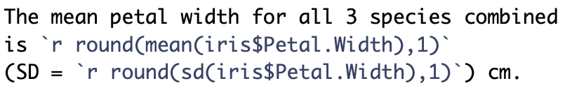
Output:

The mean petal width for all 3 species combined is 1.2 (SD = 0.8) cm.

• Reporting summary statistics this way in a report, makes the numbers computationally reproducible.
• For example, if this were for an abstract and a year later you are wondering where the numbers came from, your R code will tell you exactly which dataset was used to calculate the values.

(1.4) Summarizing numerical data - Day 3 in F24

Measures of center & spread

https://xkcd.com/937/

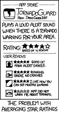
Table 1 example

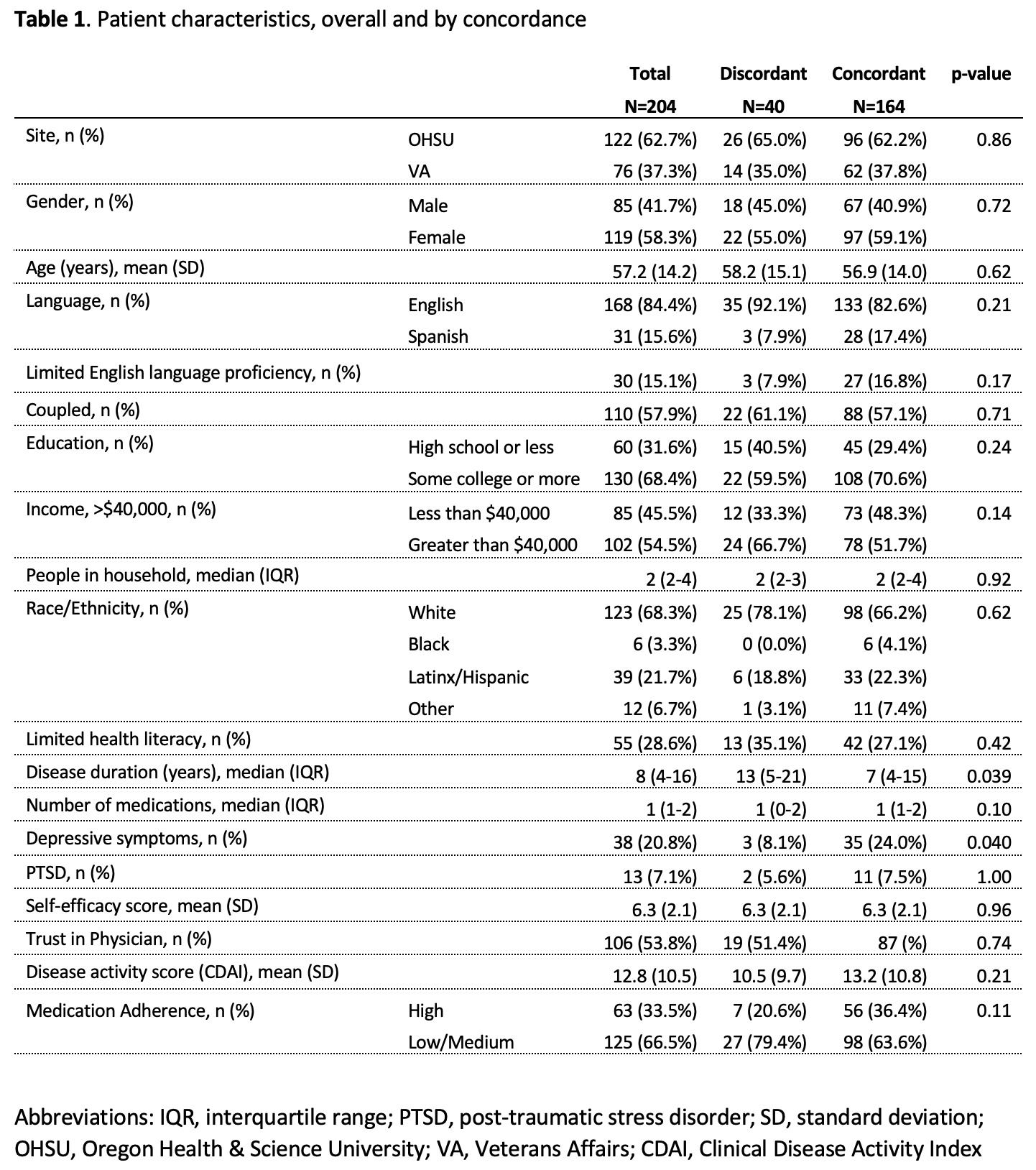
Are We on the Same Page?: A Cross-Sectional Study of Patient-Clinician Goal Concordance in Rheumatoid Arthritis
J Barton et al.
Arthritis Care & Research.
2021 Sep 27 https://pubmed.ncbi.nlm.nih.gov/34569172/

Measures of center: mean

Sample mean: the average value of observations

\[\overline{x} = \frac{x_1+x_2+\cdots+x_n}{n} = \sum_{i=1}^{n}\frac{x_i}{n}\]

where \(x_1, x_2, \ldots, x_n\) represent the \(n\) observed values in a sample

Example: What is the mean age in the toy dataset df defined earlier?

df

  IDs gender  age     trt Veteran
1   1   male 28.0 control   FALSE
2   2 female 35.5       1    TRUE
3   3   Male 31.0       1    TRUE

mean(df$age)

[1] 31.5

Measures of center: median

• The median is the middle value of the observations in a sample.

• The median is the 50th percentile, meaning

  • 50% of observations lie below and
  • 50% of observations lie above the median.

• If the number of observations is
  • odd: the median is the middle observed value
  • even: the median is the average of the two middle observed values

df$age

[1] 28.0 35.5 31.0

median(df$age)

[1] 31

median(c(df$age, 67))

[1] 33.25

Measures of center: mean vs. median

`stat_bin()` using `bins = 30`. Pick better value with `binwidth`.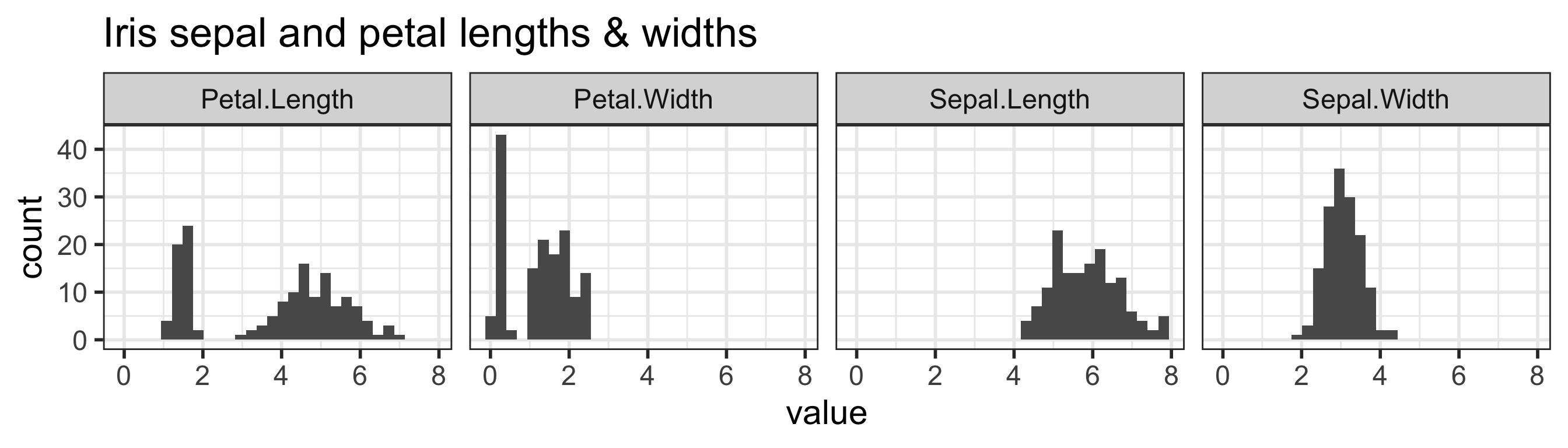

summary(iris)

  Sepal.Length    Sepal.Width     Petal.Length    Petal.Width   
 Min.   :4.300   Min.   :2.000   Min.   :1.000   Min.   :0.100  
 1st Qu.:5.100   1st Qu.:2.800   1st Qu.:1.600   1st Qu.:0.300  
 Median :5.800   Median :3.000   Median :4.350   Median :1.300  
 Mean   :5.843   Mean   :3.057   Mean   :3.758   Mean   :1.199  
 3rd Qu.:6.400   3rd Qu.:3.300   3rd Qu.:5.100   3rd Qu.:1.800  
 Max.   :7.900   Max.   :4.400   Max.   :6.900   Max.   :2.500  
       Species  
 setosa    :50  
 versicolor:50  
 virginica :50  
                
                
                

Measures of center: mode

mode: the most frequent value in a dataset

`stat_bin()` using `bins = 30`. Pick better value with `binwidth`.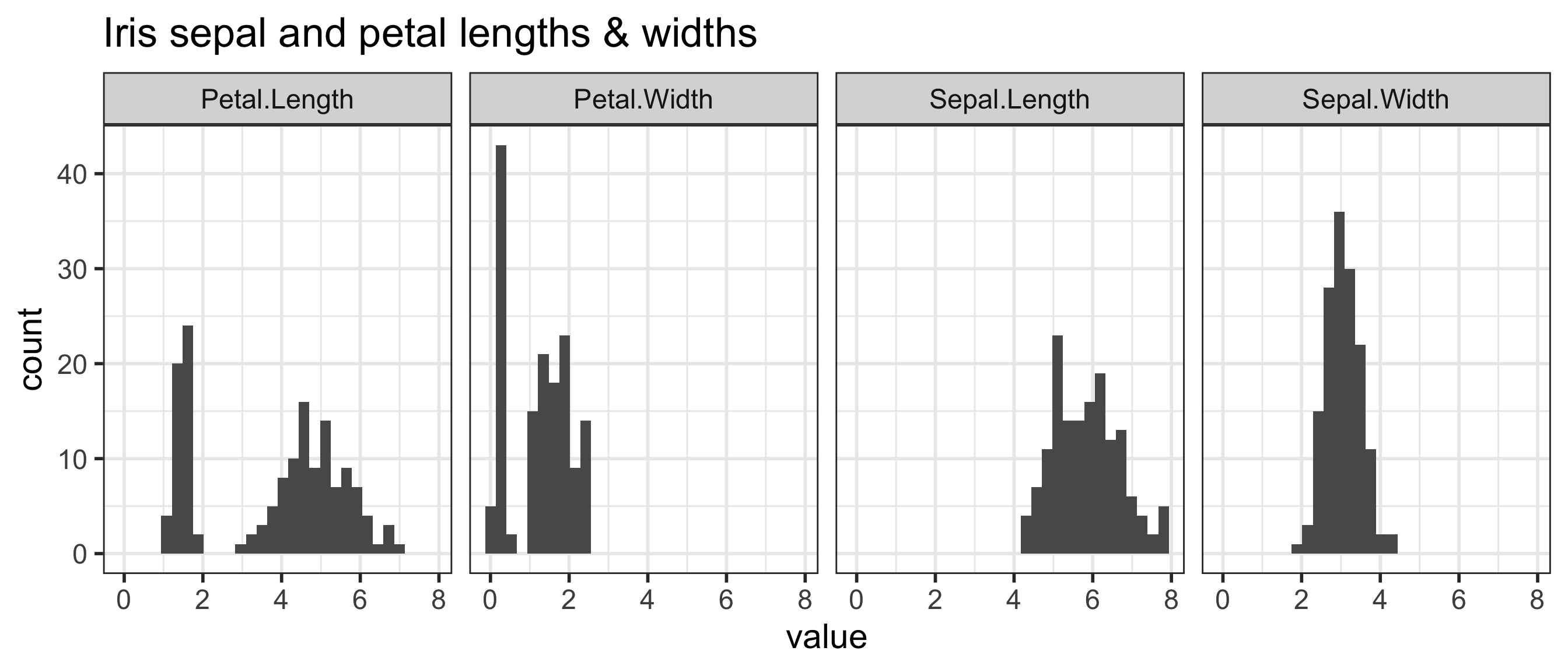

Measures of spread: standard deviation (SD) (1/3)

standard deviation is (approximately) the average distance between a typical observation and the mean

• An observation’s deviation is the distance between its value \(x\) and the sample mean \(\overline{x}\): deviation = \(x - \overline{x}\).

`stat_bin()` using `bins = 30`. Pick better value with `binwidth`.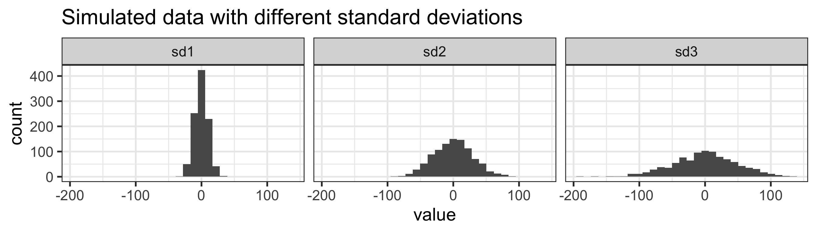

Measures of spread: SD (2/3)

• The sample variance \(s^2\) is the sum of squared deviations divided by the number of observations minus 1. \[s^2 = \frac{(x_1 - \overline{x})^2+(x_2 - \overline{x})^2+\cdots+(x_n - \overline{x})^2}{n-1} = \sum_{i=1}^{n}\frac{(x_i - \overline{x})^2}{n-1}\] where \(x_1, x_2, \dots, x_n\) represent the \(n\) observed values.

• The standard deviation \(s\) is the square root of the variance. \[s = \sqrt{\frac{({x_1 - \overline{x})}^{2}+({x_2 - \overline{x})}^{2}+\cdots+({x_n - \overline{x})}^{2}}{n-1}} = \sqrt{\sum_{i=1}^{n}\frac{(x_i - \overline{x})^2}{n-1}}\]

Measures of spread: SD (3/3)

Let’s calculate the sample standard deviation for our toy example

df$age

[1] 28.0 35.5 31.0

mean(df$age)

[1] 31.5

sd(df$age)

[1] 3.774917

\(s = \sqrt{\sum_{i=1}^{n}\frac{(x_i - \overline{x})^2}{n-1}} =\)

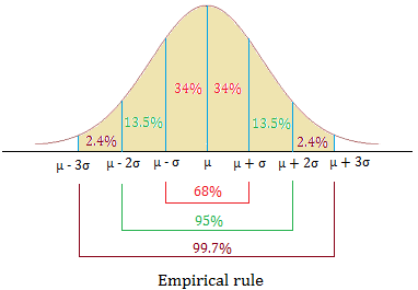
Empirical Rule: one way to think about the SD (1/2)

For symmetric bell-shaped data, about

• 68% of the data are within 1 SD of the mean
• 95% of the data are within 2 SD’s of the mean
• 99.7% of the data are within 3 SD’s of the mean

These percentages are based off of percentages of a true normal distribution.

https://statistics-made-easy.com/empirical-rule/

Empirical Rule: one way to think about the SD (2/2)

hist(iris$Sepal.Width)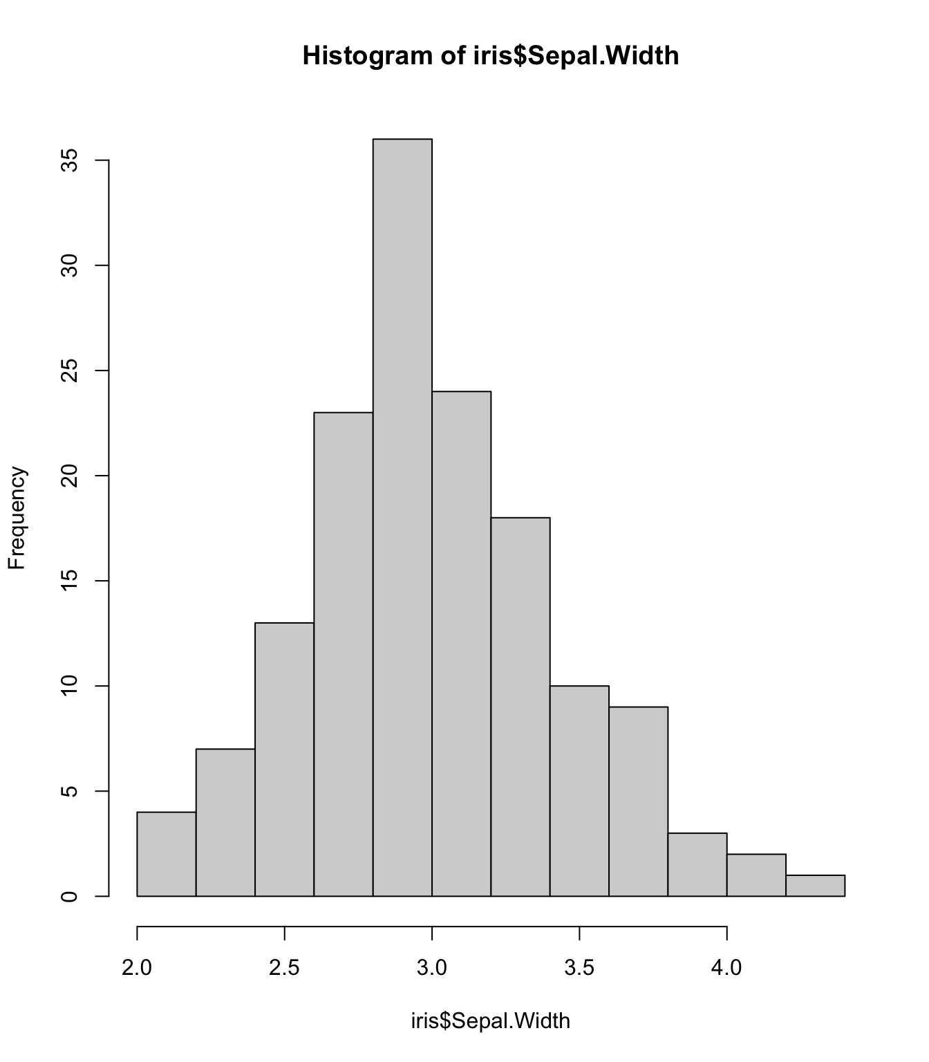

mean(iris$Sepal.Width)

[1] 3.057333

sd(iris$Sepal.Width)

[1] 0.4358663

Measures of spread: interquartile range (IQR) (1/2)

The \(p^{th}\) percentile is the observation such that \(p\%\) of the remaining observations fall below this observation.

• The first quartile \(Q_1\) is the \(25^{th}\) percentile.
• The second quartile \(Q_2\), i.e., the median, is the \(50^{th}\) percentile.
• The third quartile \(Q_3\) is the \(75^{th}\) percentile.

The interquartile range (IQR) is the distance between the third and first quartiles. \[IQR = Q_3 - Q_1\]

• IQR is the width of the middle half of the data

Measures of spread: IQR (2/2)

5 number summary

summary(iris$Sepal.Width)

   Min. 1st Qu.  Median    Mean 3rd Qu.    Max. 
  2.000   2.800   3.000   3.057   3.300   4.400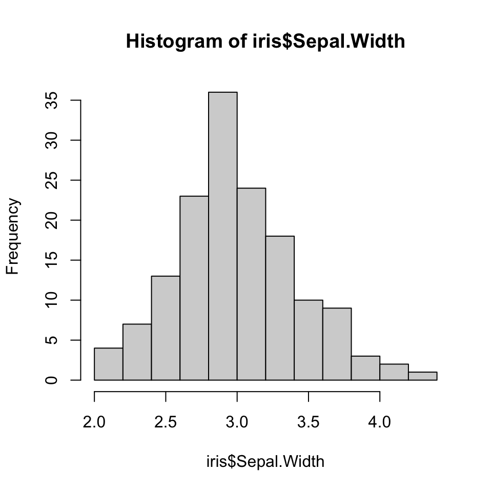 

What is the IQR of the sepal widths?

quantile(iris$Sepal.Width, c(.25, .75))

25% 75% 
2.8 3.3 

diff(quantile(iris$Sepal.Width, c(.25, .75)))

75% 
0.5 

IQR(iris$Sepal.Width)

[1] 0.5

Robust estimates

Summary statistics are called robust estimates if extreme observations have little effect on their values

estimate	robust?
mean
median
mode
standard deviation
IQR
range

R Packages - Day 4 in F24

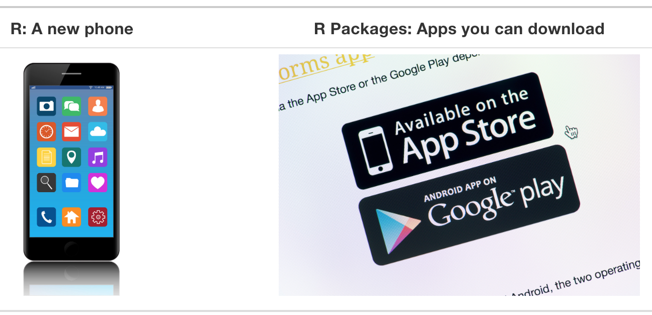
R Packages

A good analogy for R packages is that they
are like apps you can download onto a mobile phone:

ModernDive Figure 1.4

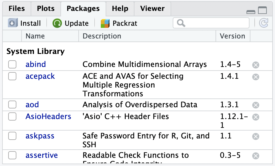
Installing packages

• Packages contain additional functions and data

Two options to install packages:

1. install.packages() or
2. The “Packages” tab in Files/Plots/Packages/Help/Viewer window

install.packages("dplyr")   # only do this ONCE, use quotes

• Only install packages once (unless you want to update them)
• Installed from Comprehensive R Archive Network (CRAN) = package mothership

Video on installing packages

• Danielle Navarro’s YouTube video on Installing and loading R packages: https://www.youtube.com/watch?v=kpHZVyDvEhQ

Load packages with library() command

• Tip: at the top of your Rmd file, create a chunk that loads all of the R packages you want to use in that file.
• Use the library() command to load each required package.
• Packages need to be reloaded every time you open Rstudio.

library(dplyr)    # run this every time you open Rstudio

• You can use a function without loading the package with PackageName::CommandName

dplyr::arrange(iris, Petal.Width)   # what does arrange do?

    Sepal.Length Sepal.Width Petal.Length Petal.Width    Species
1            4.9         3.1          1.5         0.1     setosa
2            4.8         3.0          1.4         0.1     setosa
3            4.3         3.0          1.1         0.1     setosa
4            5.2         4.1          1.5         0.1     setosa
5            4.9         3.6          1.4         0.1     setosa
6            5.1         3.5          1.4         0.2     setosa
7            4.9         3.0          1.4         0.2     setosa
8            4.7         3.2          1.3         0.2     setosa
9            4.6         3.1          1.5         0.2     setosa
10           5.0         3.6          1.4         0.2     setosa
11           5.0         3.4          1.5         0.2     setosa
12           4.4         2.9          1.4         0.2     setosa
13           5.4         3.7          1.5         0.2     setosa
14           4.8         3.4          1.6         0.2     setosa
15           5.8         4.0          1.2         0.2     setosa
16           5.4         3.4          1.7         0.2     setosa
17           4.6         3.6          1.0         0.2     setosa
18           4.8         3.4          1.9         0.2     setosa
19           5.0         3.0          1.6         0.2     setosa
20           5.2         3.5          1.5         0.2     setosa
21           5.2         3.4          1.4         0.2     setosa
22           4.7         3.2          1.6         0.2     setosa
23           4.8         3.1          1.6         0.2     setosa
24           5.5         4.2          1.4         0.2     setosa
25           4.9         3.1          1.5         0.2     setosa
26           5.0         3.2          1.2         0.2     setosa
27           5.5         3.5          1.3         0.2     setosa
28           4.4         3.0          1.3         0.2     setosa
29           5.1         3.4          1.5         0.2     setosa
30           4.4         3.2          1.3         0.2     setosa
31           5.1         3.8          1.6         0.2     setosa
32           4.6         3.2          1.4         0.2     setosa
33           5.3         3.7          1.5         0.2     setosa
34           5.0         3.3          1.4         0.2     setosa
35           4.6         3.4          1.4         0.3     setosa
36           5.1         3.5          1.4         0.3     setosa
37           5.7         3.8          1.7         0.3     setosa
38           5.1         3.8          1.5         0.3     setosa
39           5.0         3.5          1.3         0.3     setosa
40           4.5         2.3          1.3         0.3     setosa
41           4.8         3.0          1.4         0.3     setosa
42           5.4         3.9          1.7         0.4     setosa
43           5.7         4.4          1.5         0.4     setosa
44           5.4         3.9          1.3         0.4     setosa
45           5.1         3.7          1.5         0.4     setosa
46           5.0         3.4          1.6         0.4     setosa
47           5.4         3.4          1.5         0.4     setosa
48           5.1         3.8          1.9         0.4     setosa
49           5.1         3.3          1.7         0.5     setosa
50           5.0         3.5          1.6         0.6     setosa
51           4.9         2.4          3.3         1.0 versicolor
52           5.0         2.0          3.5         1.0 versicolor
53           6.0         2.2          4.0         1.0 versicolor
54           5.8         2.7          4.1         1.0 versicolor
55           5.7         2.6          3.5         1.0 versicolor
56           5.5         2.4          3.7         1.0 versicolor
57           5.0         2.3          3.3         1.0 versicolor
58           5.6         2.5          3.9         1.1 versicolor
59           5.5         2.4          3.8         1.1 versicolor
60           5.1         2.5          3.0         1.1 versicolor
61           6.1         2.8          4.7         1.2 versicolor
62           5.8         2.7          3.9         1.2 versicolor
63           5.5         2.6          4.4         1.2 versicolor
64           5.8         2.6          4.0         1.2 versicolor
65           5.7         3.0          4.2         1.2 versicolor
66           5.5         2.3          4.0         1.3 versicolor
67           5.7         2.8          4.5         1.3 versicolor
68           6.6         2.9          4.6         1.3 versicolor
69           5.6         2.9          3.6         1.3 versicolor
70           6.1         2.8          4.0         1.3 versicolor
71           6.4         2.9          4.3         1.3 versicolor
72           6.3         2.3          4.4         1.3 versicolor
73           5.6         3.0          4.1         1.3 versicolor
74           5.5         2.5          4.0         1.3 versicolor
75           5.6         2.7          4.2         1.3 versicolor
76           5.7         2.9          4.2         1.3 versicolor
77           6.2         2.9          4.3         1.3 versicolor
78           5.7         2.8          4.1         1.3 versicolor
79           7.0         3.2          4.7         1.4 versicolor
80           5.2         2.7          3.9         1.4 versicolor
81           6.1         2.9          4.7         1.4 versicolor
82           6.7         3.1          4.4         1.4 versicolor
83           6.6         3.0          4.4         1.4 versicolor
84           6.8         2.8          4.8         1.4 versicolor
85           6.1         3.0          4.6         1.4 versicolor
86           6.1         2.6          5.6         1.4  virginica
87           6.4         3.2          4.5         1.5 versicolor
88           6.9         3.1          4.9         1.5 versicolor
89           6.5         2.8          4.6         1.5 versicolor
90           5.9         3.0          4.2         1.5 versicolor
91           5.6         3.0          4.5         1.5 versicolor
92           6.2         2.2          4.5         1.5 versicolor
93           6.3         2.5          4.9         1.5 versicolor
94           6.0         2.9          4.5         1.5 versicolor
95           5.4         3.0          4.5         1.5 versicolor
96           6.7         3.1          4.7         1.5 versicolor
97           6.0         2.2          5.0         1.5  virginica
98           6.3         2.8          5.1         1.5  virginica
99           6.3         3.3          4.7         1.6 versicolor
100          6.0         2.7          5.1         1.6 versicolor
101          6.0         3.4          4.5         1.6 versicolor
102          7.2         3.0          5.8         1.6  virginica
103          6.7         3.0          5.0         1.7 versicolor
104          4.9         2.5          4.5         1.7  virginica
105          5.9         3.2          4.8         1.8 versicolor
106          6.3         2.9          5.6         1.8  virginica
107          7.3         2.9          6.3         1.8  virginica
108          6.7         2.5          5.8         1.8  virginica
109          6.5         3.0          5.5         1.8  virginica
110          6.3         2.7          4.9         1.8  virginica
111          7.2         3.2          6.0         1.8  virginica
112          6.2         2.8          4.8         1.8  virginica
113          6.1         3.0          4.9         1.8  virginica
114          6.4         3.1          5.5         1.8  virginica
115          6.0         3.0          4.8         1.8  virginica
116          5.9         3.0          5.1         1.8  virginica
117          5.8         2.7          5.1         1.9  virginica
118          6.4         2.7          5.3         1.9  virginica
119          7.4         2.8          6.1         1.9  virginica
120          5.8         2.7          5.1         1.9  virginica
121          6.3         2.5          5.0         1.9  virginica
122          6.5         3.2          5.1         2.0  virginica
123          5.7         2.5          5.0         2.0  virginica
124          5.6         2.8          4.9         2.0  virginica
125          7.7         2.8          6.7         2.0  virginica
126          7.9         3.8          6.4         2.0  virginica
127          6.5         3.0          5.2         2.0  virginica
128          7.1         3.0          5.9         2.1  virginica
129          7.6         3.0          6.6         2.1  virginica
130          6.8         3.0          5.5         2.1  virginica
131          6.7         3.3          5.7         2.1  virginica
132          6.4         2.8          5.6         2.1  virginica
133          6.9         3.1          5.4         2.1  virginica
134          6.5         3.0          5.8         2.2  virginica
135          7.7         3.8          6.7         2.2  virginica
136          6.4         2.8          5.6         2.2  virginica
137          6.4         3.2          5.3         2.3  virginica
138          7.7         2.6          6.9         2.3  virginica
139          6.9         3.2          5.7         2.3  virginica
140          7.7         3.0          6.1         2.3  virginica
141          6.9         3.1          5.1         2.3  virginica
142          6.8         3.2          5.9         2.3  virginica
143          6.7         3.0          5.2         2.3  virginica
144          6.2         3.4          5.4         2.3  virginica
145          5.8         2.8          5.1         2.4  virginica
146          6.3         3.4          5.6         2.4  virginica
147          6.7         3.1          5.6         2.4  virginica
148          6.3         3.3          6.0         2.5  virginica
149          7.2         3.6          6.1         2.5  virginica
150          6.7         3.3          5.7         2.5  virginica

Install the packages listed below before Day 3

• knitr
  • this might actually already be installed
  • check your packages list
• tidyverse
  • this is actually a bundle of packages
  • Warning: it will take a while to install!!!
  • see more info at https://tidyverse.tidyverse.org/
• rstatix
  • for summary statistics of a dataset
• janitor
  • for cleaning and exploring data
• ggridges
  • for creating ridgeline plots
• devtools
  • used to create R packages
  • for our purposes, needed to install some packages
• oi_biostat_data
  • this package is on github
  • see the next slide for directions on how to install oi_biostat_data

Directions for installing package oibiostat

• The textbook’s datasets are in the R package oibiostat
• Explanation of code below
  • Installation of oibiostat package requires first installing devtools package
  • The code devtools::install_github() tells R to use the command install_github() from the devtools package without loading the entire package and all of its commands (which library(devtools) would do).

install.packages("devtools")
devtools::install_github("OI-Biostat/oi_biostat_data", force = TRUE)

• After running the code above, put # in front of the commands so that RStudio doesn’t evaluate them when rendering.
• Now load the oibiostat package
  • the code below needs to be run every time you restart R or knit an Rmd file

library(oibiostat)

A visual dataset

Compare water sources across the world by country and family income

Gapminder Dollarstreet

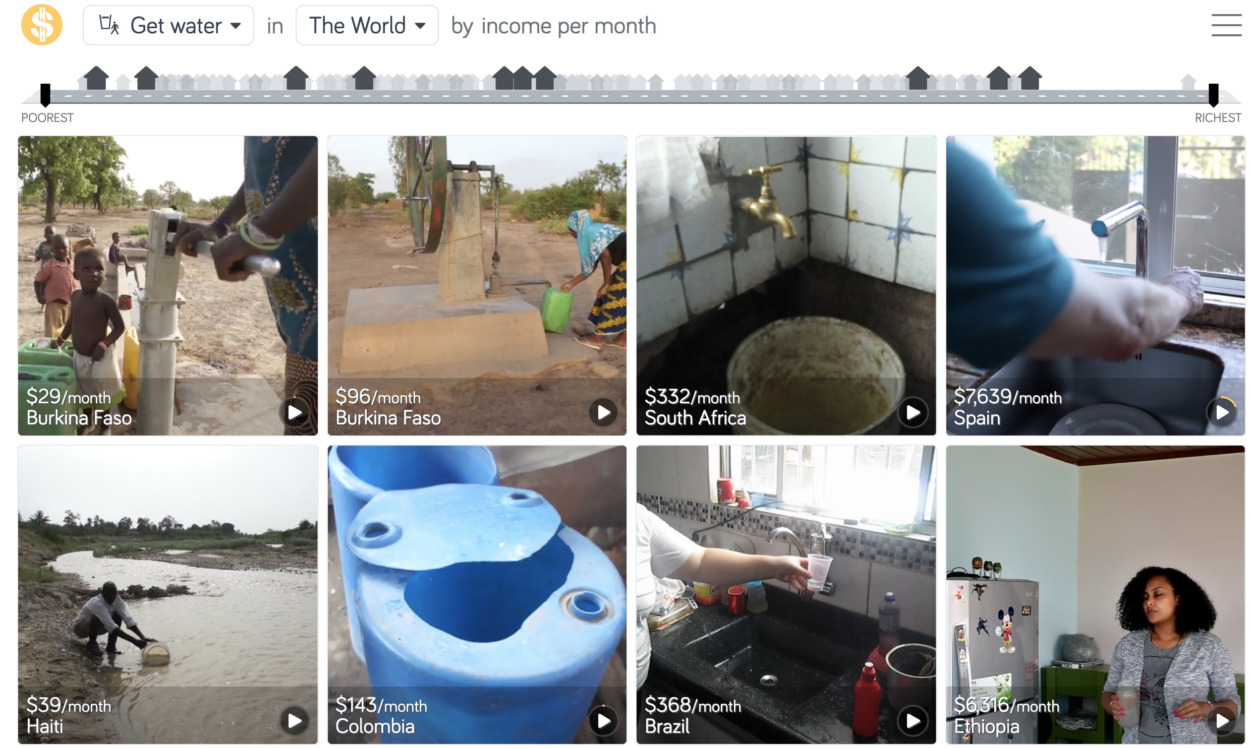
Check out Gapminder’s Dollar Street for many more examples: https://www.gapminder.org/dollar-street