Day 1: Intro to R & Rstudio

BSTA 511/611 Fall 2024, OHSU

Week 1

Author

Meike Niederhausen, PhD

Published

October 2, 2024

Introduction to R

What is R?

A programming language
Focus on statistical modeling and data analysis
- import data, manipulate data, run statistics, make plots
Useful for data science
Great visualizations
Also useful for most anything else you’d want to tell a computer to do
Interfaces with other languages i.e. python, C++, bash

For the history and details: Wikipedia

an interpreted language (run it through a command line)
procedural programming with functions
Why “R”?? Scheme inspired S (invented at Bell Labs in 1976) which inspired R since 1st letters of original authors (free and open source! in 2000)

What is RStudio?

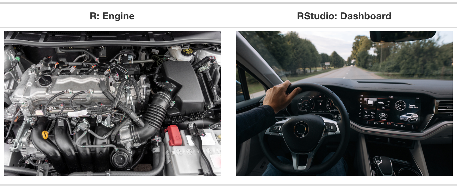
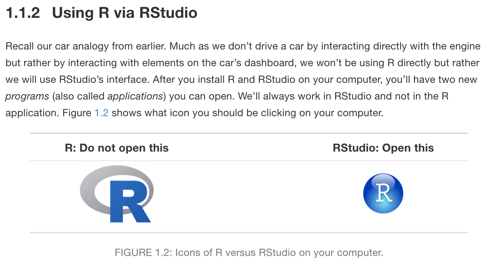
R is a programming language

RStudio is an integrated development environment (IDE)
= an interface to use R (with perks!)

Open RStudio on your computer (not R!)

RStudio anatomy

Read more about RStudio’s layout in Section 3.4 of “Getting Used to R, RStudio, and R Markdown” (Ismay and Kennedy 2016)

Let’s code! R Basics

Coding in the console

When you first open R, the console should be empty.

Typing and executing code in the console

Type code in the console (blue text)
Press return to execute the code
Output shown below in black

Math calculations using R

Rules for order of operations are followed
Spaces between numbers and characters are ignored

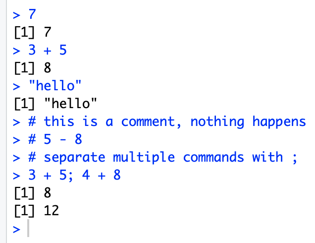
10^2

[1] 100

3 ^ 7

[1] 2187

6/9

[1] 0.6666667

9-43

[1] -34

4^3-2* 7+9 /2

[1] 54.5

The equation above is computed as \[4^3 − (2 \cdot 7) + \frac{9}{2}\]

Variables (saved R objects)

Variables are used to store data, figures, model output, etc.

Can assign a variable using either = or <-
- Using <- is preferable

Assign just one value:

x = 5
x

[1] 5

x <- 5
x

[1] 5

Assign a vector of values

Consecutive integers using :

a <- 3:10
a

[1]  3  4  5  6  7  8  9 10

Concatenate a string of numbers

b <- c(5, 12, 2, 100, 8)
b

[1]   5  12   2 100   8

Doing math with variables

Math using variables with just one value

x <- 5
x

[1] 5

x + 3

[1] 8

y <- x^2
y

[1] 25

Math on vectors of values:
element-wise computation

a <- 3:6
a

[1] 3 4 5 6

a+2; a*3

[1] 5 6 7 8

[1]  9 12 15 18

a*a

[1]  9 16 25 36

Variables can include text (characters)

hi <- "hello"
hi

[1] "hello"

greetings <- c("Guten Tag", "Hola", hi)
greetings

[1] "Guten Tag" "Hola"      "hello"

Using functions

mean() is an example of a function
functions have “arguments” that can be specified within the ()
?mean in console will show help file for mean()

Function arguments specified by name:

mean(x = 1:4)

[1] 2.5

seq(from = 1, to = 12, by = 3)

[1]  1  4  7 10

seq(by = 3, to = 12, from = 1)

[1]  1  4  7 10

Function arguments not specified, but listed in order:

mean(1:4)

[1] 2.5

seq(1, 12, 3)

[1]  1  4  7 10

Common console errors (1/2)

Incomplete commands

When the console is waiting for a new command, the prompt line begins with >
- If the console prompt is +, then a previous command is incomplete
- You can finish typing the command in the console window

Example:

> 3 + (2*6
+ )

[1] 15

Common console errors (2/2)

Object is not found

This happens when text is entered for a non-existent variable (object)

Example:

hello

Error in eval(expr, envir, enclos): object 'hello' not found

Can be due to missing quotes

install.packages(dplyr)

Error in install.packages(dplyr): object 'dplyr' not found

# correct code is: install.packages("dplyr")

Saving your work with Quarto

or, creating reproducible reports

Example: creating an html file

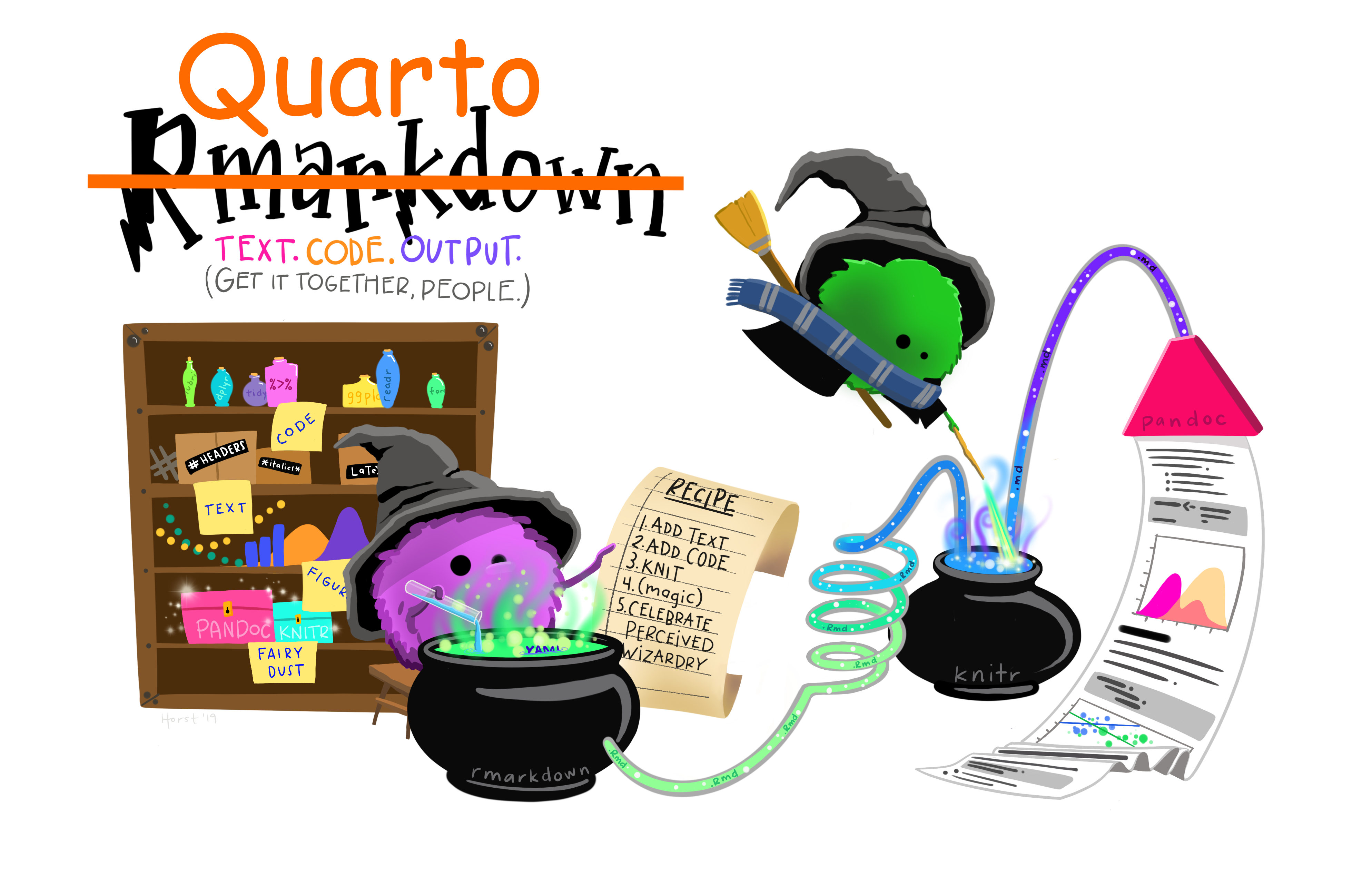
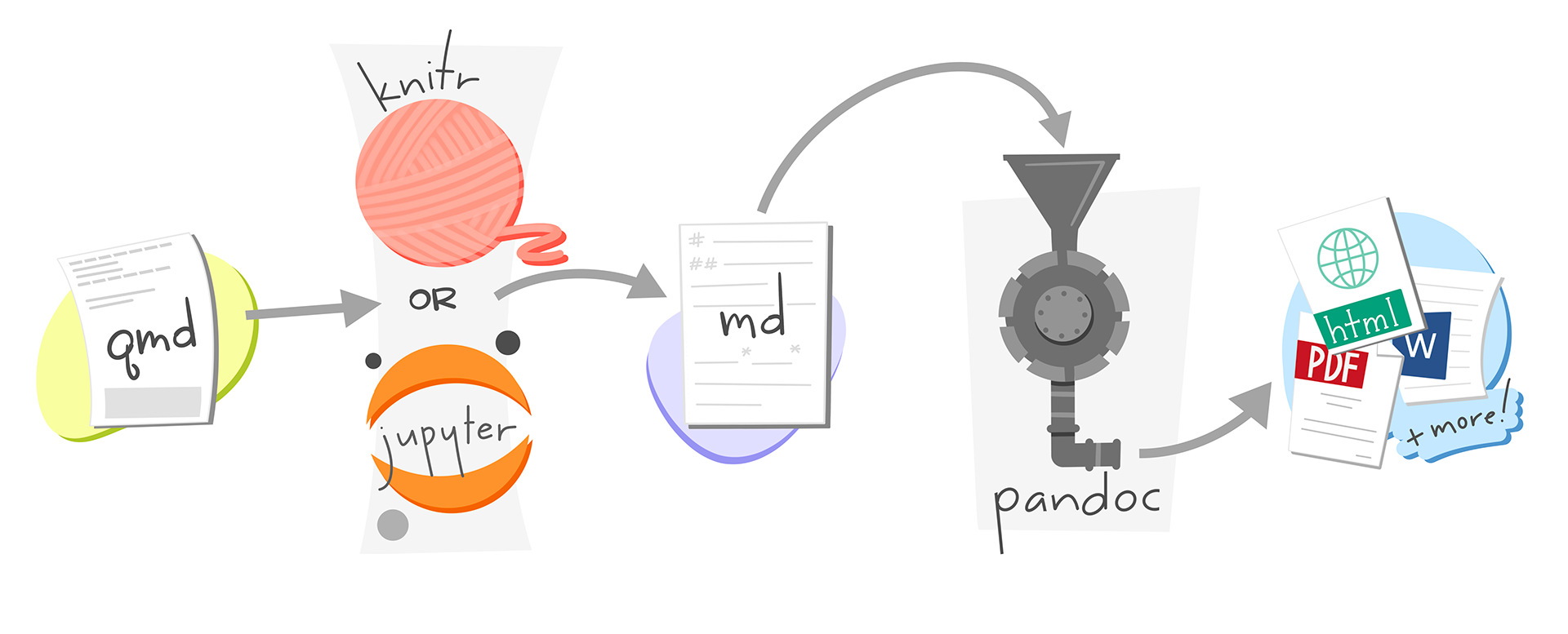
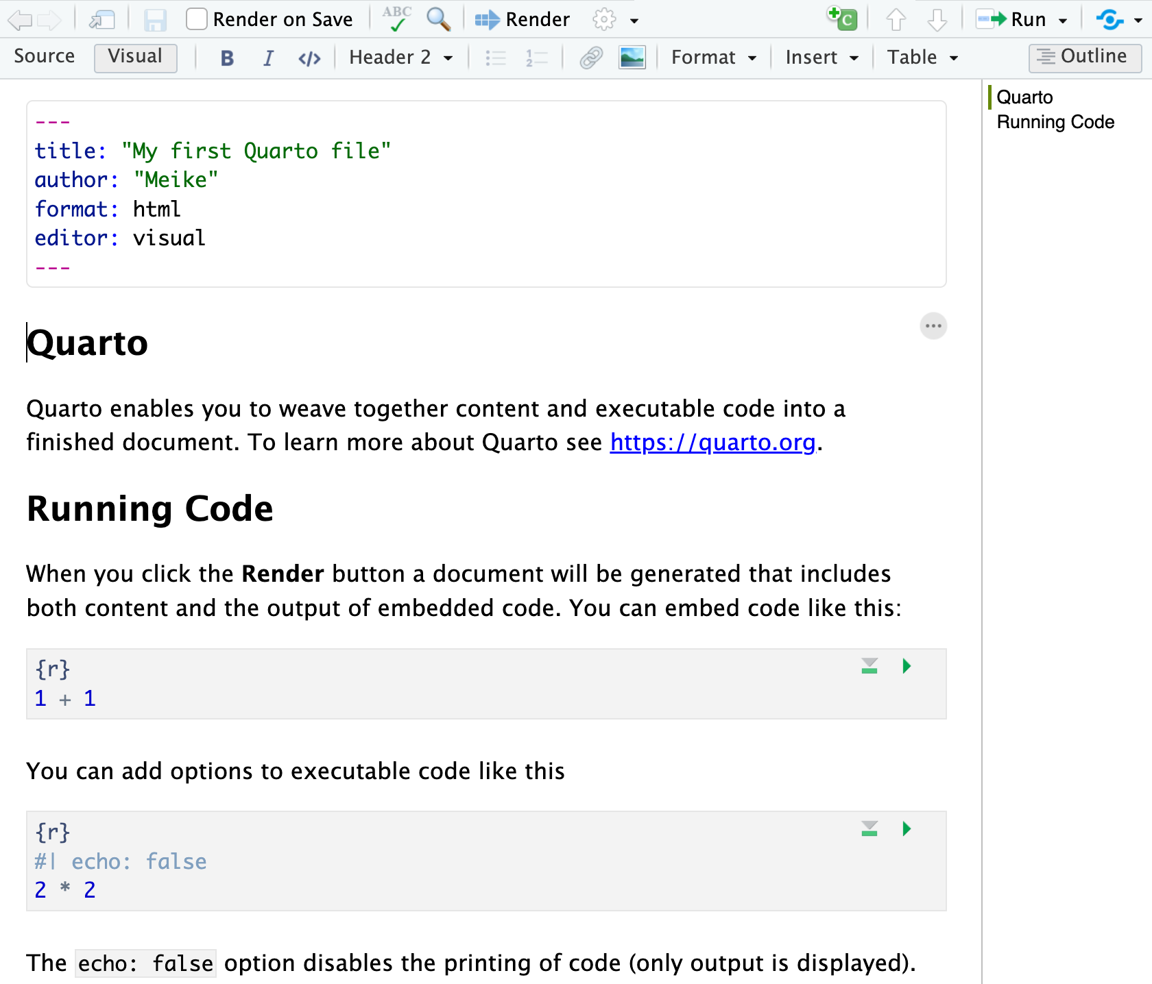
.qmd file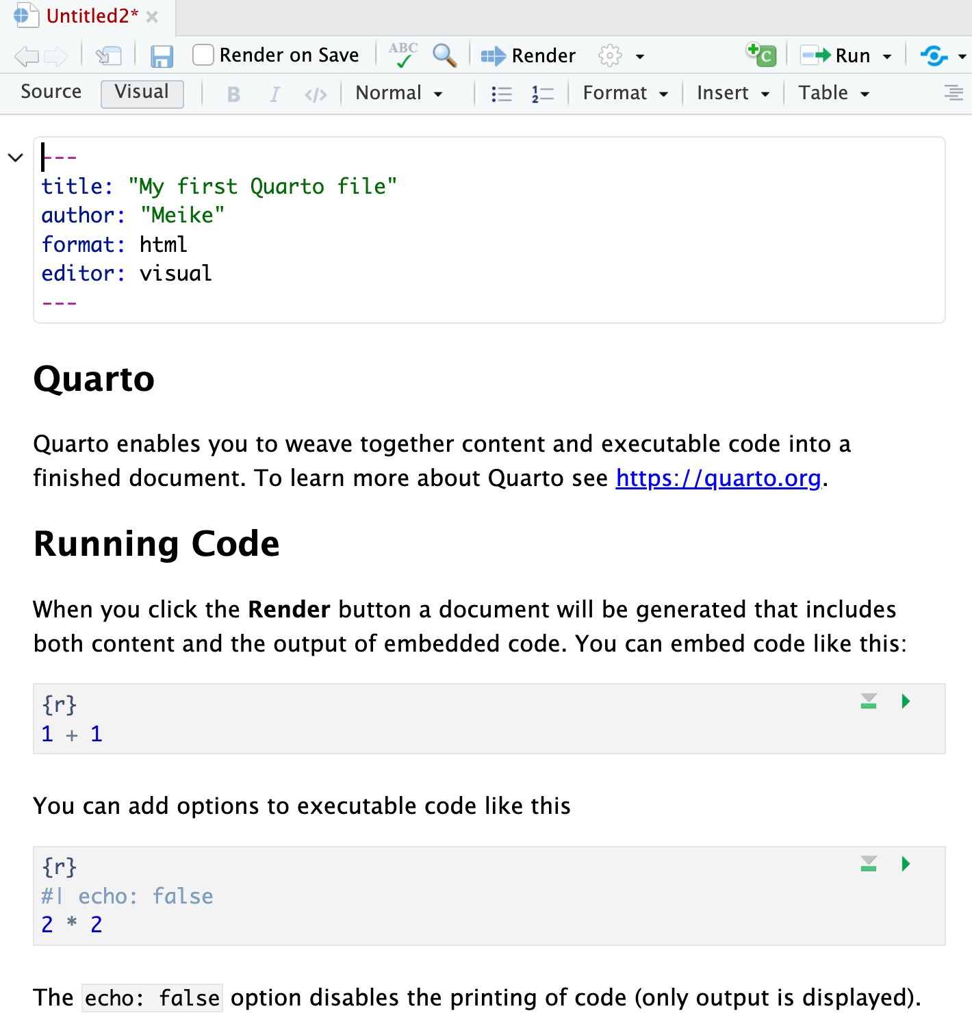

html output

Quarto = `.qmd` file = Code + text

knitr is a package that converts .qmd files containing code + markdown syntax to a plain text .md markdown file, and then to other formats (html, pdf, Word, etc)

Artwork from “Hello, Quarto” keynote by Julia Lowndes and Mine Çetinkaya-Rundel, presented at RStudio Conference 2022. Illustrated by Allison Horst.

Basic Quarto example

1. Create a Quarto file (`.qmd`)

Two options:

click on File \(\rightarrow\) New File \(\rightarrow\) Quarto Document…\(\rightarrow\) OK,
or in upper left corner of RStudio click on \(\rightarrow\)

Pop-up window selections:

Enter a title and your name
Select HTML output format (default)
Engine: select Knitr
Editor: Select Use visual markdown editor
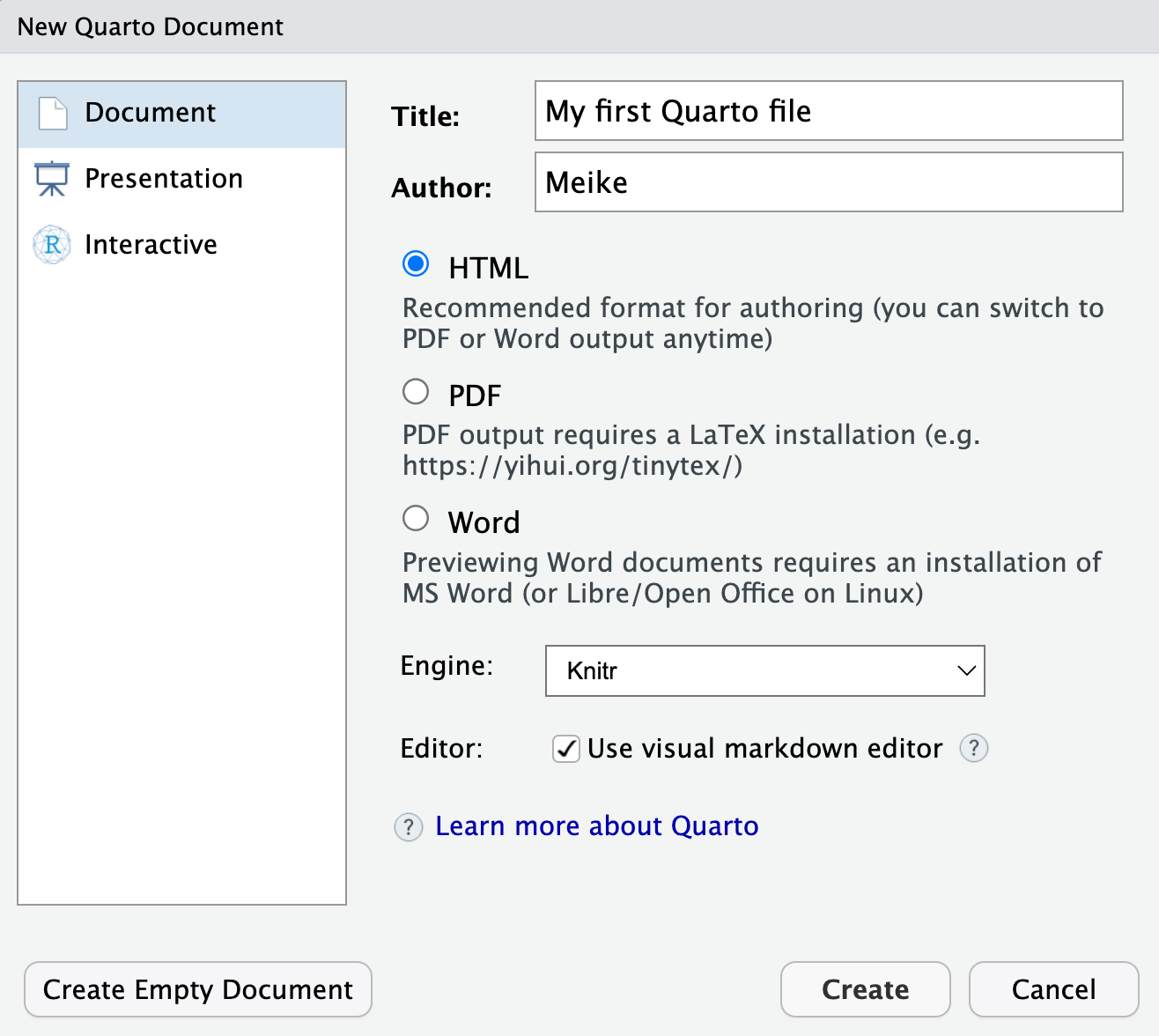
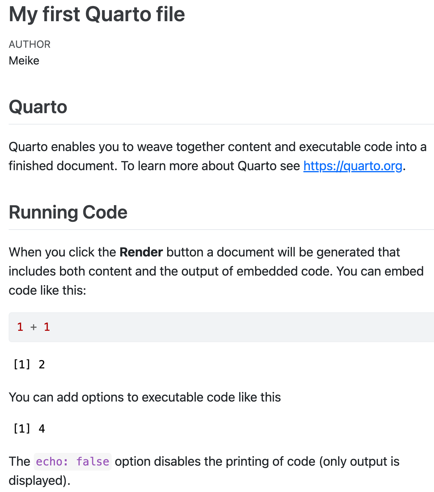
Click Create

2. Create a Quarto file (`.qmd`)

After clicking on Create, you should then see the following in your editor window:

3. Save the Quarto file (`.qmd`)

Save the file by
- selecting File -> Save,
- or clicking on (towards the left above the scripting window),
- or keyboard shortcut
  - PC: Ctrl + s
  - Mac: Command + s
You will need to specify
- a filename to save the file as
  - ALWAYS use .qmd as the filename extension for Quarto files
- the folder to save the file in

4. Create html file

We create the html file by rendering the .qmd file.

Two options:

click on the Render icon at the top of the editor window,
or use keyboard shortcuts
- Mac: Command+Shift+K
- PC: Ctrl+Shift+K

A new window will open with the html output.
You will now see both .qmd and .html files in the folder where you saved the .qmd file.

Note

The template .qmd file that RStudio creates will render to an html file by default.
The output format can be changed to create a Word doc, pdf, slides, etc.

.qmd file vs. its html output

.qmd file

html output

3 types of Quarto content

Text, lists, images, tables, links
Code chunks
YAML metadata

Illustration by Alison Hill and Allison Horst, for RStudio.

Formatting text

bold, italics, super^scripts & sub_scripts, ~~strikethrough~~, verbatim, etc.
Text is formatted through a markup language called Markdown (Wikipedia)
- Other markup languages include html (webapges) and LaTeX (math)
- All text formatting is specified via code
- “Markdown is a plain text format that is designed to be easy to write, and, even more importantly, easy to read” ¹
Newer versions of RStudio include a Visual editor as well that makes formatting text similar to using a word processor.

Formatting text: `Visual editor`

Using the Visual editor is similar to using a wordprocessor, such as Word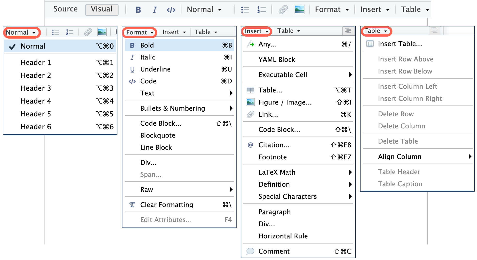
Keyboard shortcuts usually work as well (shown for Mac below)

Practice

Part 1
1. Using the visual editor, practice formatting text in your qmd file, such as making text bold, italicized, and in code format.
2. Add 1^st, 2^nd, and 3^rd level headers
3. Add a list with a
  - sub-list (bullet and/or numbered)
4. Add a table
5. Add whatever else you are interested in!
Part 2
1. Switch back to the Source editor and examine the markdown code that was used for the formatting.

Questions:

What went smoothly?
What hurdles did you encounter?

Formatting text: `Markdown`

Markdown:	Output:
`This text is in italics, but _so is this text_.`	This text is in italics, but so is this text.
`Bold also has __2 options__`	Bold also has 2 options
`~~Should this be deleted?~~`	~~Should this be deleted?~~
`Need^super^ or~sub~ scripts?`	Need^super or_sub scripts?
`Code is often formatted as verbatim`	`Code is often formatted as verbatim`
`>This is a block quote.`	This is a block quote.

Headers

Organize your documents using headers to create sections and subsections
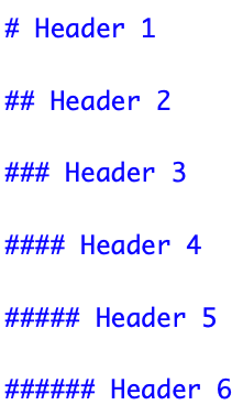
Use # at the beginning of the line to create headers

Text in editor:

Output:

Important

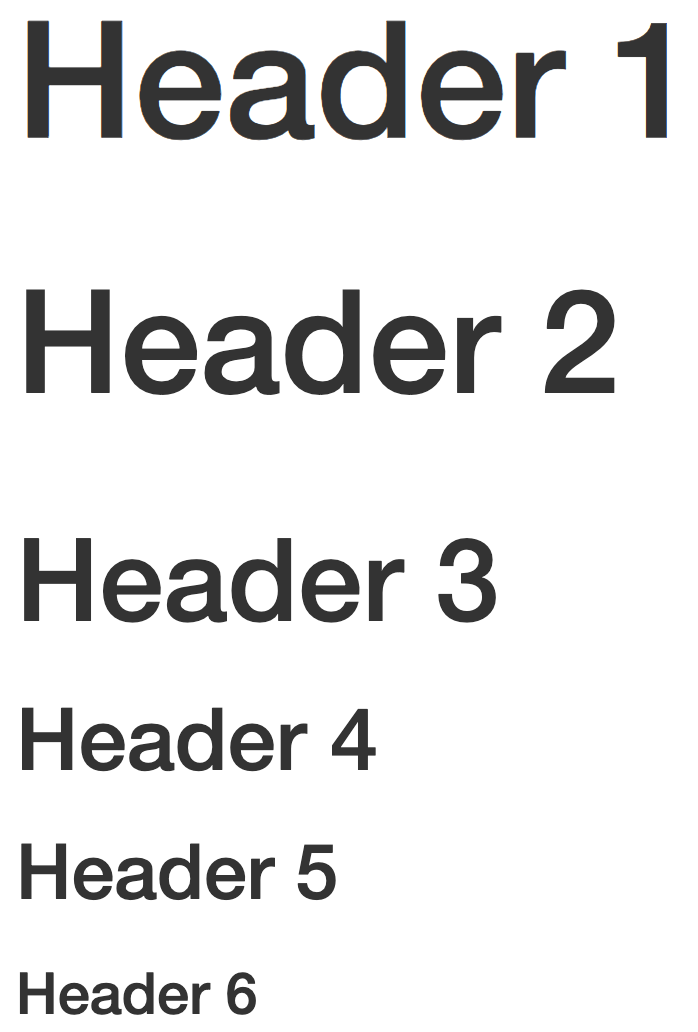
Make sure there is no space before the #, and there IS a space after the # in order for the header to work properly.

RStudio tip

You can easily navigate through your .qmd file if you use headers to outline your text

3 types of Quarto content

Text, lists, images, tables, links
Code chunks
YAML metadata

Code chunks

.qmd file

html output

Create a code chunk

3 options to create a code chunk

Click on at top right of the editor window, or
Keyboard shortcut

Mac	Command + Option + I
PC	Ctrl + Alt + I

Visual editor: Select Insert -> Executable Cell -> R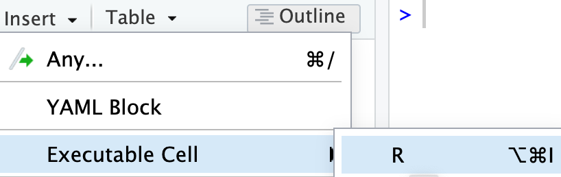

What does a code chunk look like?

An empty code chunk looks like this:

Visual editor

Source editor

Important

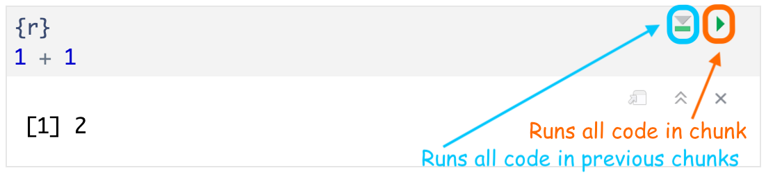
Note that a code chunks start with ```{r} and ends with ```. Make sure there is no space before ```.

Enter and run code (1/n)

Type R code inside code chunks
Select code you want to run, by
- placing the cursor in the line of code you want to run,
- or highlighting the code you want to run

Run selected code by
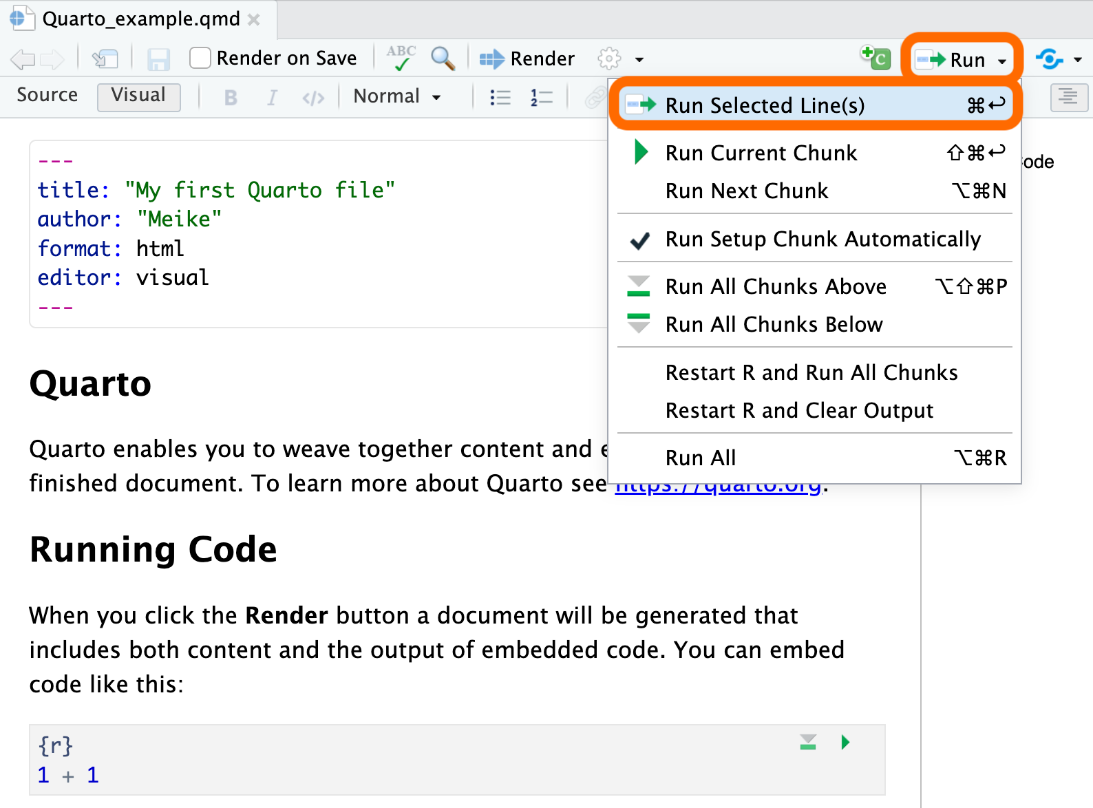
- clicking on the button in the top right corner of the scripting window and choosing Run Selected Line(s),
- or typing one of the following key combinations:

Mac	ctrl + return
PC	command + return

Where does the output appear?

Enter and run code (2/n)

Run all code in a chunk by
- by clicking the play button in the top right corner of the chunk
The code output appears below the code chunk

Note

The output should also appear in the Console.
Settings can be changed so that the output appears only in the Console and not below the code chunk:
- Select (to right of Render button) and then Chunk Output in Console.

Useful keyboard shortcuts

Full list of keyboard shortcuts

action	mac	windows/linux
Run code in qmd (or script)	cmd + enter	ctrl + enter
`<-`	option + -	alt + -
interrupt currently running command	esc	esc
in console, retrieve previously run code	up/down	up/down
keyboard shortcut help	option + shift + k	alt + shift + k

Practice

Try typing code below in your qmd (with shortcut) and evaluating it:

y <- 5
y

3 types of Quarto content

Text, lists, images, tables, links
Code chunks
YAML metadata

`YAML` metadata

Many output options can be set in the YAML metadata, which is the first set of code in the file starting and ending with ---.

It sets the configuration specifications for the output file
YAML is an acronym for
- yet another markup language, or
- YAML ain’t markup language

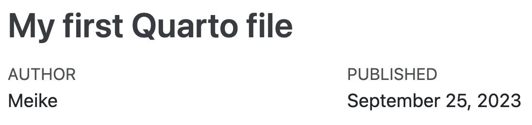
Simple `YAML` example

The default YAML includes a title and author that appear at the top of the output file. In the example below, I also added in a date option

YAML:

---
title: "My first Quarto file"
author: "Meike"
date: "9/25/2023"
format: html
editor: visual
---

Output:

Important

The YAML must start and end with 3 dashes ---.
The first set of --- must be on the very first line.

Change the output file type

The YAML specifies the format of the output file:
- html, Word, pdf, slides, website, book, etc.
This is done by changing the format: option

---
title: "My first Quarto file"
author: "Meike"
date: "9/25/2023"
format: html
editor: visual
---

Output format	YAML
html	`format: html`
Word	`format: docx`
pdf²	`format: pdf`
html slides	`format: revealjs`
PPT slides	`format: pptx`

You WILL get frustrated while learning R!

From Garrett Grolemund’s Prologue of his book Hands-On Programming with R³:

As you learn to program, you are going to get frustrated. You are learning a new language, and it will take time to become fluent. But frustration is not just natural, it’s actually a positive sign that you should watch for. Frustration is your brain’s way of being lazy; it’s trying to get you to quit and go do something easy or fun. If you want to get physically fitter, you need to push your body even though it complains. If you want to get better at programming, you’ll need to push your brain. Recognize when you get frustrated and see it as a good thing: you’re now stretching yourself. Push yourself a little further every day, and you’ll soon be a confident programmer.

Resources

Official Quarto guide: https://quarto.org/docs/guide/
- Markdown basics: https://quarto.org/docs/authoring/markdown-basics.html
  - Text formatting, headings, linnks, images, lists, tables, equations, diagrams, page breaks, keyboard shortcuts, and more!
- Code blocks: https://quarto.org/docs/computations/r.html#code-blocks
  - Chunk options: https://quarto.org/docs/computations/r.html#chunk-options
Mine Çetinkaya-Rundel’s Quarto tip a day: https://mine-cetinkaya-rundel.github.io/quarto-tip-a-day/
Hadley Wickham’s R for Data Science: https://r4ds.hadley.nz/ _ See Chapter 29 for Quarto

Footnotes

From Quarto’s Markdown Basics webpage, https://quarto.org/docs/authoring/markdown-basics.html↩︎
requires LaTeX installation↩︎
Grolemund, Garrett. 2014. Hands-on Programming with R. O’Reilly. https://rstudio-education.github.io/hopr/↩︎

Introduction to R

What is R?

What is RStudio?

Open RStudio on your computer (not R!)

RStudio anatomy

Let’s code! R Basics

Coding in the console

Math calculations using R

Variables (saved R objects)

Doing math with variables

Variables can include text (characters)

Using functions

Common console errors (1/2)

Common console errors (2/2)

Saving your work with Quarto

Example: creating an html file

Quarto = .qmd file = Code + text

Basic Quarto example

1. Create a Quarto file (.qmd)

2. Create a Quarto file (.qmd)

3. Save the Quarto file (.qmd)

4. Create html file

.qmd file vs. its html output

3 types of Quarto content

Formatting text

Formatting text: Visual editor

Practice

Formatting text: Markdown

Headers

RStudio tip

3 types of Quarto content

Code chunks

Create a code chunk

What does a code chunk look like?

Enter and run code (1/n)

Enter and run code (2/n)

Useful keyboard shortcuts

Practice

3 types of Quarto content

YAML metadata

Simple YAML example

Change the output file type

You WILL get frustrated while learning R!

Resources

Footnotes

Quarto = `.qmd` file = Code + text

1. Create a Quarto file (`.qmd`)

2. Create a Quarto file (`.qmd`)

3. Save the Quarto file (`.qmd`)

Formatting text: `Visual editor`

Formatting text: `Markdown`

`YAML` metadata

Simple `YAML` example