Day 14: Comparing Means with ANOVA (Section 5.5)

BSTA 511/611

Week 8

Author

Affiliation

Meike Niederhausen, PhD

OHSU-PSU School of Public Health

Published

November 20, 2024

Load packages

Packages need to be loaded every time you restart R or render an Qmd file

# run these every time you open Rstudio
library(tidyverse)    
library(oibiostat)
library(janitor)
library(rstatix)
library(knitr)
library(gtsummary)
library(moderndive)
library(gt)
library(broom) 
library(here) 
library(pwr) # new-ish

You can check whether a package has been loaded or not
- by looking at the Packages tab and
- seeing whether it has been checked off or not

Goals for today (Section 5.5)

Analysis of Variance (ANOVA)
When to use an ANOVA
Hypotheses
ANOVA table
Different sources of variation in ANOVA
ANOVA conditions
F-distribution
Post-hoc testing of differences in means
Running an ANOVA in R

Disability Discrimination Example

The U.S. Rehabilitation Act of 1973 prohibited discrimination against people with physical disabilities.
- The act defined a disabled person as any individual who has a physical or mental impairment that limits the person’s major life activities.
A 1980’s study examined whether physical disabilities affect people’s perceptions of employment qualifications
- (Cesare, Tannenbaum, & Dalessio, 1990). ]
Researchers prepared recorded job interviews, using same actors and script each time.
Only difference: job applicant appeared with different disabilities.
- No disability
- Leg amputation
- Crutches
- Hearing impairment
- Wheelchair confinement
70 undergrad students were randomly assigned to view one of the videotapes,
- then rated the candidate’s qualifications on a 1-10 scale.
The research question: are qualifications evaluated differently depending on the applicant’s presented disability?

Load interview data from `.txt` file

.txt files are usually tab-deliminated files
- .csv files are comma-separated files
read_delim is from the readr package, just like read_csv

employ <- read_delim(
  file = here::here("data", "DisabilityEmployment.txt"), 
  delim = "\t",   # tab delimited
  trim_ws = TRUE)

trim_ws: Should leading and trailing whitespace be trimmed from each field before parsing it?

summary(employ)

  disability            score      
 Length:70          Min.   :1.400  
 Class :character   1st Qu.:3.700  
 Mode  :character   Median :5.050  
                    Mean   :4.929  
                    3rd Qu.:6.100  
                    Max.   :8.500

employ %>% tabyl(disability)

 disability  n percent
    amputee 14     0.2
   crutches 14     0.2
    hearing 14     0.2
       none 14     0.2
 wheelchair 14     0.2

Factor variable: Make `disability` variable a factor variable

glimpse(employ)

Rows: 70
Columns: 2
$ disability <chr> "none", "none", "none", "none", "none", "none", "none", "no…
$ score      <dbl> 1.9, 2.5, 3.0, 3.6, 4.1, 4.2, 4.9, 5.1, 5.4, 5.9, 6.1, 6.7,…

summary(employ)

  disability            score      
 Length:70          Min.   :1.400  
 Class :character   1st Qu.:3.700  
 Mode  :character   Median :5.050  
                    Mean   :4.929  
                    3rd Qu.:6.100  
                    Max.   :8.500

Make disability a factor variable:

employ <- employ %>% 
  mutate(disability = factor(disability))

What’s different now?

glimpse(employ)

Rows: 70
Columns: 2
$ disability <fct> none, none, none, none, none, none, none, none, none, none,…
$ score      <dbl> 1.9, 2.5, 3.0, 3.6, 4.1, 4.2, 4.9, 5.1, 5.4, 5.9, 6.1, 6.7,…

summary(employ)

      disability     score      
 amputee   :14   Min.   :1.400  
 crutches  :14   1st Qu.:3.700  
 hearing   :14   Median :5.050  
 none      :14   Mean   :4.929  
 wheelchair:14   3rd Qu.:6.100  
                 Max.   :8.500

Factor variable: Change order & name of disability levels

What are the current level names and order?

levels(employ$disability)

[1] "amputee"    "crutches"   "hearing"    "none"       "wheelchair"

What changes are being made below?

employ <- employ %>% 
  mutate(
    # make "none" the first level
    # by only listing the level none, all other levels will be in original order
    disability = fct_relevel(disability, "none"),
    # change the level name amputee to amputation
    disability = fct_recode(disability, amputation = "amputee")
    )

fct_relevel() and fct_recode() are from the forcats package: https://forcats.tidyverse.org/index.html.
forcats is loaded with library(tidyverse).

New order & names:

levels(employ$disability) # note the new order and new name

[1] "none"       "amputation" "crutches"   "hearing"    "wheelchair"

Data viz

What are the score distribution shapes within each group?
Any unusual values?

ggplot(employ, aes(x=score)) +
  geom_density() +
  facet_wrap(~ disability)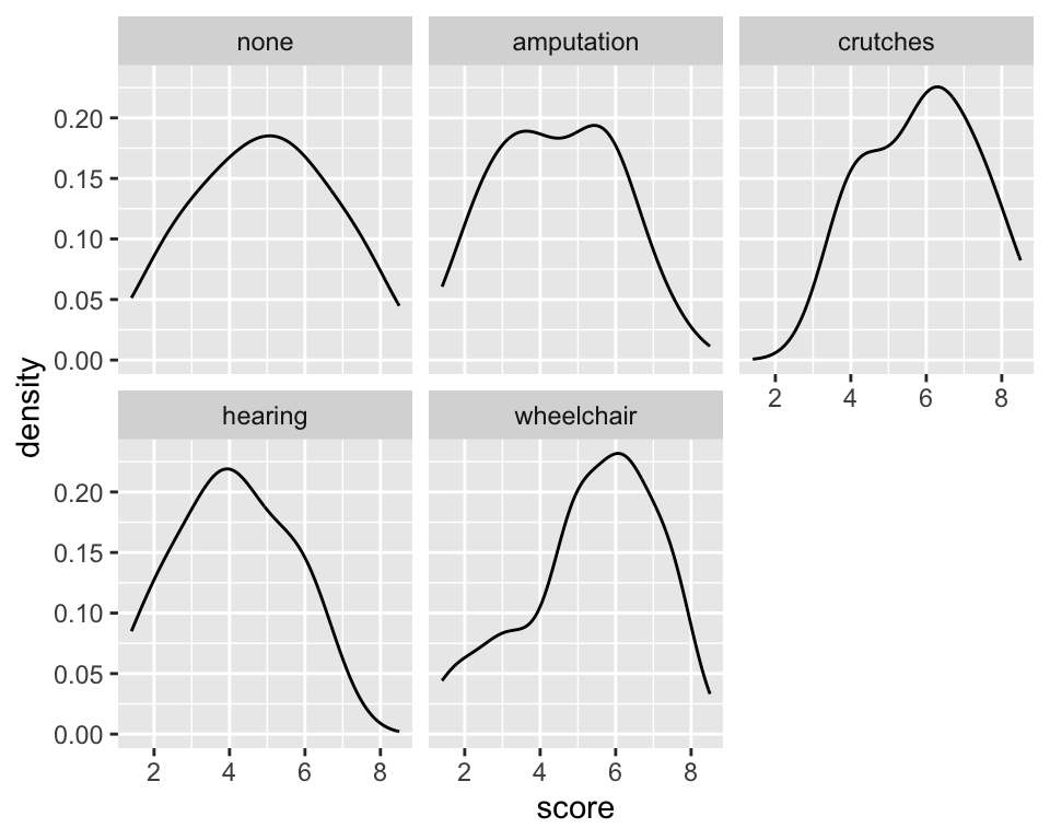

library(ggridges) 
ggplot(employ, 
       aes(x=score,
           y = disability,
           fill = disability)) + 
  geom_density_ridges(alpha = 0.4) +
  theme(legend.position="none")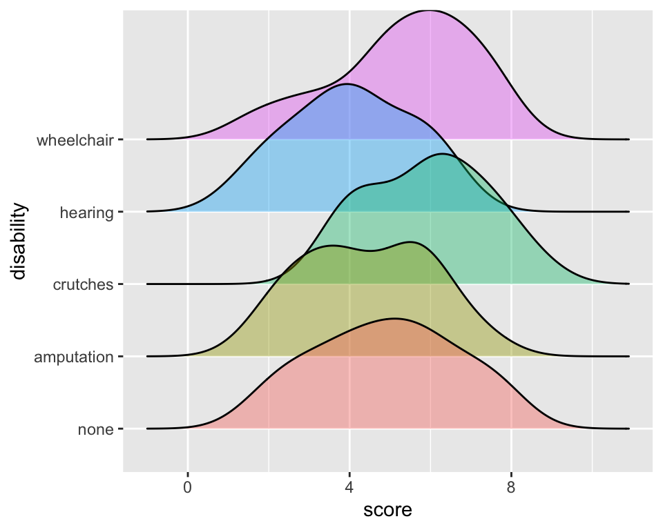

Compare the score measures of center and spread between the groups

ggplot(employ, aes(y=score, x = disability,
                   fill = disability)) +
  geom_boxplot(alpha =.3) +
  coord_flip() +
  geom_jitter(width =.1, alpha = 0.3) +
  theme(legend.position = "none")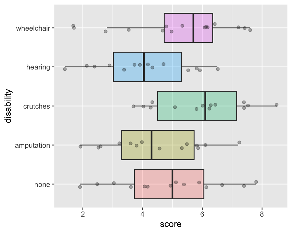

ggplot(employ, aes(x = disability, y=score, 
    fill=disability, color=disability)) +
  geom_dotplot(binaxis = "y", alpha =.5) +
  geom_hline(aes(yintercept = mean(score)), 
             lty = "dashed") +
  stat_summary(fun ="mean", geom="point", 
    size = 3, color = "grey33", alpha =1) +
  theme(legend.position = "none")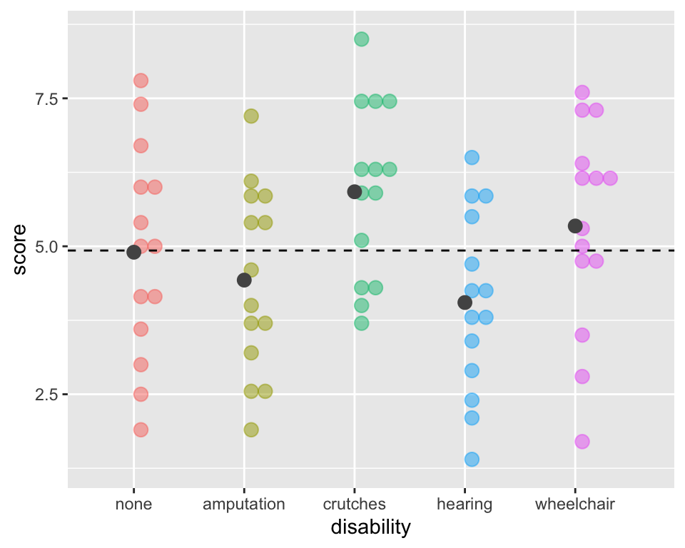

ANOVA

Hypotheses

To test for a difference in means across k groups:

\[\begin{align} H_0 &: \mu_1 = \mu_2 = ... = \mu_k\\ \text{vs. } H_A&: \text{At least one pair } \mu_i \neq \mu_j \text{ for } i \neq j \end{align}\]

Hypothetical examples:
In which set (A or B) do you believe the evidence will be stronger that at least one population differs from the others?

See slides

Comparing means

Whether or not two means are significantly different depends on:

How far apart the means are
How much variability there is within each group

Questions:

How to measure variability between groups?
How to measure variability within groups?
How to compare the two measures of variability?
How to determine significance?

ANOVA in base R

There are several options to run an ANOVA model in R
Two most common are lm and aov
- lm = linear model; will be using frequently in BSTA 512

lm(score ~ disability, data = employ) %>% anova()

Analysis of Variance Table

Response: score
           Df  Sum Sq Mean Sq F value  Pr(>F)  
disability  4  30.521  7.6304  2.8616 0.03013 *
Residuals  65 173.321  2.6665                  
---
Signif. codes:  0 '***' 0.001 '**' 0.01 '*' 0.05 '.' 0.1 ' ' 1

aov(score ~ disability, data = employ) %>% summary()

            Df Sum Sq Mean Sq F value Pr(>F)  
disability   4  30.52   7.630   2.862 0.0301 *
Residuals   65 173.32   2.666                 
---
Signif. codes:  0 '***' 0.001 '**' 0.01 '*' 0.05 '.' 0.1 ' ' 1

Hypotheses:

\[\begin{align} H_0 &: \mu_{none} = \mu_{amputation} = \mu_{crutches} = \mu_{hearing} = \mu_{wheelchair}\\ \text{vs. } H_A&: \text{At least one pair } \mu_i \neq \mu_j \text{ for } i \neq j \end{align}\]

Do we reject or fail to reject \(H_0\)?

ANOVA tables

See slides

ANOVA: Analysis of Variance

Analysis of Variance (ANOVA) compares the variability between groups to the variability within groups

\[\sum_{i = 1}^k \sum_{j = 1}^{n_i}(x_{ij} -\bar{x})^2 \ \ = \ \sum_{i = 1}^k n_i(\bar{x}_{i}-\bar{x})^2 \ \ + \ \ \sum_{i = 1}^k\sum_{j = 1}^{n_i}(x_{ij}-\bar{x}_{i})^2\]

Notation

k groups
\(n_i\) observations in each of the k groups
Total sample size is \(N=\sum_{i=1}^{k}n_i\)
\(\bar{x}_{i}\) = mean of observations in group i
\(\bar{x}\) = mean of all observations
\(s_{i}\) = sd of observations in group i
\(s\) = sd of all observations

Observation	i = 1	i = 2	i = 3	\(\ldots\)	i = k	overall
j = 1	\(x_{11}\)	\(x_{21}\)	\(x_{31}\)	\(\ldots\)	\(x_{k1}\)
j = 2	\(x_{12}\)	\(x_{22}\)	\(x_{32}\)	\(\ldots\)	\(x_{k2}\)
j = 3	\(x_{13}\)	\(x_{23}\)	\(x_{33}\)	\(\ldots\)	\(x_{k3}\)
j = 4	\(x_{14}\)	\(x_{24}\)	\(x_{34}\)	\(\ldots\)	\(x_{k4}\)
\(\vdots\)	\(\vdots\)	\(\vdots\)	\(\vdots\)	\(\ddots\)	\(\vdots\)
j = \(n_i\)	\(x_{1n_1}\)	\(x_{2n_2}\)	\(x_{3n_3}\)	\(\ldots\)	\(x_{kn_k}\)
Means	\(\bar{x}_{1}\)	\(\bar{x}_{2}\)	\(\bar{x}_{3}\)	\(\ldots\)	\(\bar{x}_{k}\)	\(\bar{x}\)
Variance	\({s}^2_{1}\)	\({s}^2_{2}\)	\({s}^2_{3}\)	\(\ldots\)	\({s}^2_{k}\)	\({s}^2\)

Total Sums of Squares Visually

ggplot(employ, aes(x = disability, y=score, 
      fill = disability, color = disability)) +
  geom_dotplot(binaxis = "y", alpha =.9) +
  geom_hline(aes(yintercept = mean(score)), 
             lty = "dashed") +
  # stat_summary(fun = "mean", geom = "point", 
  #      size = 3, color = "grey33", alpha =1)  +
  theme(legend.position = "none")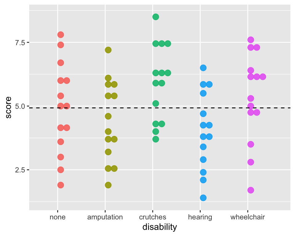

Total Sums of Squares:

\[SST = \sum_{i = 1}^k \sum_{j = 1}^{n_i}(x_{ij} -\bar{x})^2 = (N-1)s^2\]

where
- \(N=\sum_{i=1}^{k}n_i\) is the total sample size and
- \(s^2\) is the grand standard deviation of all the observations
This is the sum of the squared differences between each observed \(x_{ij}\) value and the grand mean, \(\bar{x}\).
That is, it is the total deviation of the \(x_{ij}\)’s from the grand mean.

Calculate Total Sums of Squares

Total Sums of Squares:

\[SST = \sum_{i = 1}^k \sum_{j = 1}^{n_i}(x_{ij} -\bar{x})^2 = (N-1)s^2\]

where
- \(N=\sum_{i=1}^{k}n_i\) is the total sample size and
- \(s^2\) is the grand standard deviation of all the observations

Total sample size \(N\):

(Ns <- employ %>% group_by(disability) %>% count())

# A tibble: 5 × 2
# Groups:   disability [5]
  disability     n
  <fct>      <int>
1 none          14
2 amputation    14
3 crutches      14
4 hearing       14
5 wheelchair    14

\(SST\):

(SST <- (sum(Ns$n) - 1) * sd(employ$score)^2)

[1] 203.8429

Sums of Squares due to Groups Visually (“between” groups)

ggplot(employ, aes(x = disability, y=score, 
      fill = disability, color = disability)) +
  geom_dotplot(binaxis = "y", alpha =.2) +
  geom_hline(aes(yintercept = mean(score)), 
             lty = "dashed") +
  stat_summary(fun = "mean", geom = "point", 
       size = 3, color = "grey33", alpha =1)  +
  theme(legend.position = "none")

Sums of Squares due to Groups:

\[SSG = \sum_{i = 1}^k n_i(\bar{x}_{i}-\bar{x})^2\]

This is the sum of the squared differences between each group mean, \(\bar{x}_{i}\), and the grand mean, \(\bar{x}\).
That is, it is the deviation of the group means from the grand mean.
Also called the Model SS, or \(SS_{model}.\)

Calculate Sums of Squares due to Groups (“between” groups)

\[SSG = \sum_{i = 1}^k n_i(\bar{x}_{i}-\bar{x})^2\]

ggplot(employ, aes(x = disability, y=score, 
      fill = disability, color = disability)) +
  geom_dotplot(binaxis = "y", alpha =.2) +
  geom_hline(aes(yintercept = mean(score)), 
             lty = "dashed") +
  stat_summary(fun = "mean", geom = "point", 
       size = 3, color = "grey33", alpha =1)  +
  theme(legend.position = "none")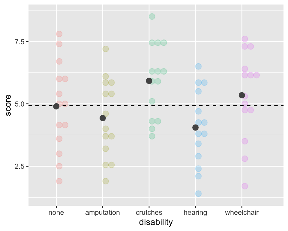

Calculate means \(\bar{x}_i\) for each group:

xbar_groups <- employ %>% 
  group_by(disability) %>% 
  summarise(mean = mean(score))
xbar_groups

# A tibble: 5 × 2
  disability  mean
  <fct>      <dbl>
1 none        4.9 
2 amputation  4.43
3 crutches    5.92
4 hearing     4.05
5 wheelchair  5.34

Calculate \(SSG\):

(SSG <- sum(Ns$n *
  (xbar_groups$mean - mean(employ$score))^2))

[1] 30.52143

Sums of Squares Error Visually (within groups)

ggplot(employ, aes(x = disability, y=score, 
      fill = disability, color = disability)) +
  geom_dotplot(binaxis = "y", alpha =.5) +
  # geom_hline(aes(yintercept = mean(score)), 
             # lty = "dashed") +
  stat_summary(fun = "mean", geom = "point", 
       size = 3, color = "grey33", alpha =1)  +
  theme(legend.position = "none")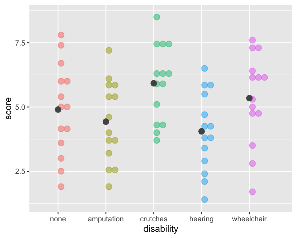

Sums of Squares Error:

\[SSE = \sum_{i = 1}^k\sum_{j = 1}^{n_i}(x_{ij}-\bar{x}_{i})^2 = \sum_{i = 1}^k(n_i-1)s_{i}^2\] where \(s_{i}\) is the standard deviation of the \(i^{th}\) group

This is the sum of the squared differences between each observed \(x_{ij}\) value and its group mean \(\bar{x}_{i}\).
That is, it is the deviation of the \(x_{ij}\)’s from the predicted score by group.
Also called the residual sums of squares, or \(SS_{residual}.\)

Calculate Sums of Squares Error (within groups)

\[SSE = \sum_{i = 1}^k\sum_{j = 1}^{n_i}(x_{ij}-\bar{x}_{i})^2 = \sum_{i = 1}^k(n_i-1)s_{i}^2\] where \(s_{i}\) is the standard deviation of the \(i^{th}\) group

ggplot(employ, aes(x = disability, y=score, 
      fill = disability, color = disability)) +
  geom_dotplot(binaxis = "y", alpha =.5) +
  # geom_hline(aes(yintercept = mean(score)), 
             # lty = "dashed") +
  stat_summary(fun = "mean", geom = "point", 
       size = 3, color = "grey33", alpha =1)  +
  theme(legend.position = "none")

Calculate sd’s \(s_i\) for each group:

sd_groups <- employ %>% 
  group_by(disability) %>% 
  summarise(SD = sd(score))
sd_groups

# A tibble: 5 × 2
  disability    SD
  <fct>      <dbl>
1 none        1.79
2 amputation  1.59
3 crutches    1.48
4 hearing     1.53
5 wheelchair  1.75

Calculate \(SSE\):

(SSE <- sum(
  (Ns$n-1)*sd_groups$SD^2))

[1] 173.3214

Verify SST = SSG + SSE

ANOVA compares the variability between groups to the variability within groups

\[\sum_{i = 1}^k \sum_{j = 1}^{n_i}(x_{ij} -\bar{x})^2 \ \ = \ \ n_i\sum_{i = 1}^k(\bar{x}_{i}-\bar{x})^2 \ \ + \ \ \sum_{i = 1}^k\sum_{j = 1}^{n_i}(x_{ij}-\bar{x}_{i})^2\]

\[(N-1)s^2 \ \ = \ \sum_{i = 1}^k n_i(\bar{x}_{i}-\bar{x})^2 \ \ + \ \ \sum_{i = 1}^k(n_i-1)s_{i}^2\]

SST

[1] 203.8429

SSG + SSE

[1] 203.8429

Thinking about the F-statistic

If the groups are actually different, then which of these is more accurate?

The variability between groups should be higher than the variability within groups
The variability within groups should be higher than the variability between groups

If there really is a difference between the groups, we would expect the F-statistic to be which of these:

Higher than we would observe by random chance
Lower than we would observe by random chance

\[F = \frac{MSG}{MSE}\]

ANOVA in base R

# Note that I'm saving the tidy anova table
# Will be pulling p-value from this on future slide

empl_lm <- lm(score ~ disability, data = employ) %>% 
  anova() %>% 
  tidy()

empl_lm %>% gt()

term	df	sumsq	meansq	statistic	p.value
disability	4	30.52143	7.630357	2.86158	0.03012686
Residuals	65	173.32143	2.666484	NA	NA

Hypotheses:

Do we reject or fail to reject \(H_0\)?

Conclusion to hypothesis test

\[\begin{align} H_0 &: \mu_{none} = \mu_{amputation} = \mu_{crutches} = \mu_{hearing} = \mu_{wheelchair}\\ \text{vs. } H_A&: \text{At least one pair } \mu_i \neq \mu_j \end{align}\]

empl_lm  # tidy anova output

# A tibble: 2 × 6
  term          df sumsq meansq statistic p.value
  <chr>      <int> <dbl>  <dbl>     <dbl>   <dbl>
1 disability     4  30.5   7.63      2.86  0.0301
2 Residuals     65 173.    2.67     NA    NA

Pull the p-value using base R:

round(empl_lm$p.value[1],2)

[1] 0.03

Pull the p-value using tidyverse:

empl_lm %>% 
  filter(term == "disability") %>% 
  pull(p.value) %>% 
  round(2)

[1] 0.03

Use \(\alpha\) = 0.05.
Do we reject or fail to reject \(H_0\)?

Conclusion statement:

There is sufficient evidence that at least one of the disability groups has a mean employment score statistically different from the other groups. ( \(p\)-value = 0.03).

Conditions for ANOVA

IF ALL of the following conditions hold:

The null hypothesis is true
Sample sizes in each group group are large (each \(n \ge 30\))
- OR the data are relatively normally distributed in each group
Variability is “similar” in all group groups:
- Is the within group variability about the same for each group?
- As a rough rule of thumb, this condition is violated if the standard deviation of one group is more than double the standard deviation of another group

THEN the sampling distribution of the
F-statistic is an F-distribution

Checking the equal variance condition:

sd_groups # previously defined

# A tibble: 5 × 2
  disability    SD
  <fct>      <dbl>
1 none        1.79
2 amputation  1.59
3 crutches    1.48
4 hearing     1.53
5 wheelchair  1.75

max(sd_groups$SD) / min(sd_groups$SD)

[1] 1.210425

Testing variances (Condition 3)

Bartlett’s test for equal variances

\(H_0:\) population variances of group levels are equal
\(H_A:\) population variances of group levels are NOT equal

Note: \(H_A\) is same as saying that at least one of the group levels has a different variance

Caution

Bartlett’s test assumes the data in each group are normally distributed.
Do not use if data do not satisfy the normality condition.

bartlett.test(score ~ disability, data = employ)


    Bartlett test of homogeneity of variances

data:  score by disability
Bartlett's K-squared = 0.7016, df = 4, p-value = 0.9511

Tip

Levene’s test for equality of variances is not as restrictive: see https://www.statology.org/levenes-test-r/

The F-distribution

The F-distribution is skewed right.
The F-distribution has two different degrees of freedom:
- one for the numerator of the ratio (k – 1) and
- one for the denominator (N – k)
\(p\)-value
- is always the upper tail
- (the area as extreme or more extreme)

F_stat <- 2.86158

ggplot(data.frame(x = c(0, 6)), aes(x = x)) + # set x-axis bounds from 0 to 6
  geom_vline(xintercept = F_stat, color = "red") +
  # fun = df is specifying (d)ensity of (f) distribution
  stat_function(fun = df, args = list(df1=4, df2=65), color = "cornflowerblue") +
  geom_area(stat = "function", fun = df, args = list(df1=4, df2=65), fill = "red", alpha =0.3, xlim = c(F_stat, 5)) +
  annotate("text", x = 3.5, y = .1, label = "p-value", size=6)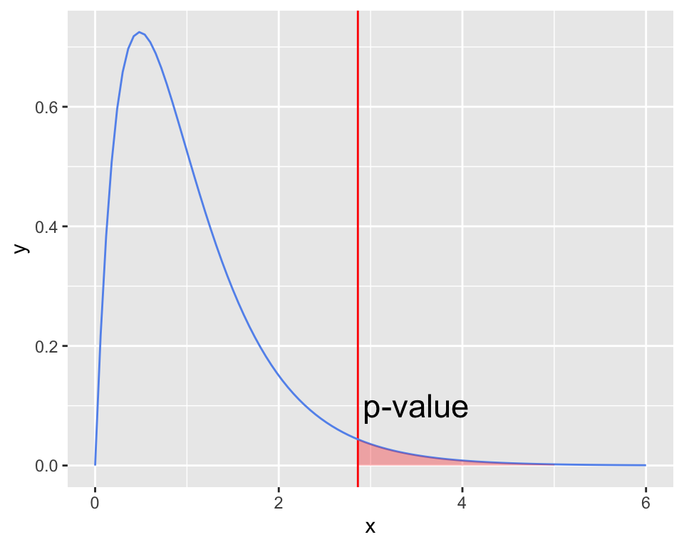

empl_lm %>% gt()

term	df	sumsq	meansq	statistic	p.value
disability	4	30.52143	7.630357	2.86158	0.03012686
Residuals	65	173.32143	2.666484	NA	NA

# p-value using F-distribution

pf(2.86158, df1=5-1, df2=70-5, 
   lower.tail = FALSE)

[1] 0.03012688

Which groups are statistically different?

So far we’ve only determined that at least one of the groups is different from the others,
- but we don’t know which.
What’s your guess?

ggplot(employ, aes(x = disability, y=score, 
      fill = disability, color = disability)) +
  geom_dotplot(binaxis = "y", alpha =.5) +
  geom_hline(aes(yintercept = mean(score)), 
             lty = "dashed") +
  stat_summary(fun = "mean", geom = "point", 
       size = 3, color = "grey33", alpha =1)  +
  theme(legend.position = "none")

Post-hoc testing for ANOVA

determining which groups are statistically different

Post-hoc testing: pairwise t-tests

In post-hoc testing we run all the pairwise t-tests comparing the means from each pair of groups.
With 5 groups, this involves doing \({5 \choose 2} = \frac{5!}{2!3!} = \frac{5\cdot 4}{2}= 10\) different pairwise tests.

Problem:

Although the ANOVA test has an \(\alpha\) chance of a Type I error (finding a difference between a pair that aren’t different),
the overall Type I error rate will be much higher when running many tests simultaneously.

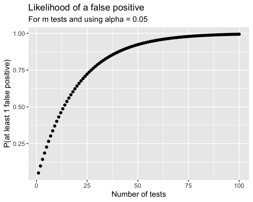
\[\begin{align} P(\text{making an error}) = & \alpha\\ P(\text{not making an error}) = & 1-\alpha\\ P(\text{not making an error in m tests}) = & (1-\alpha)^m\\ P(\text{making at least 1 error in m tests}) = & 1-(1-\alpha)^m \end{align}\]

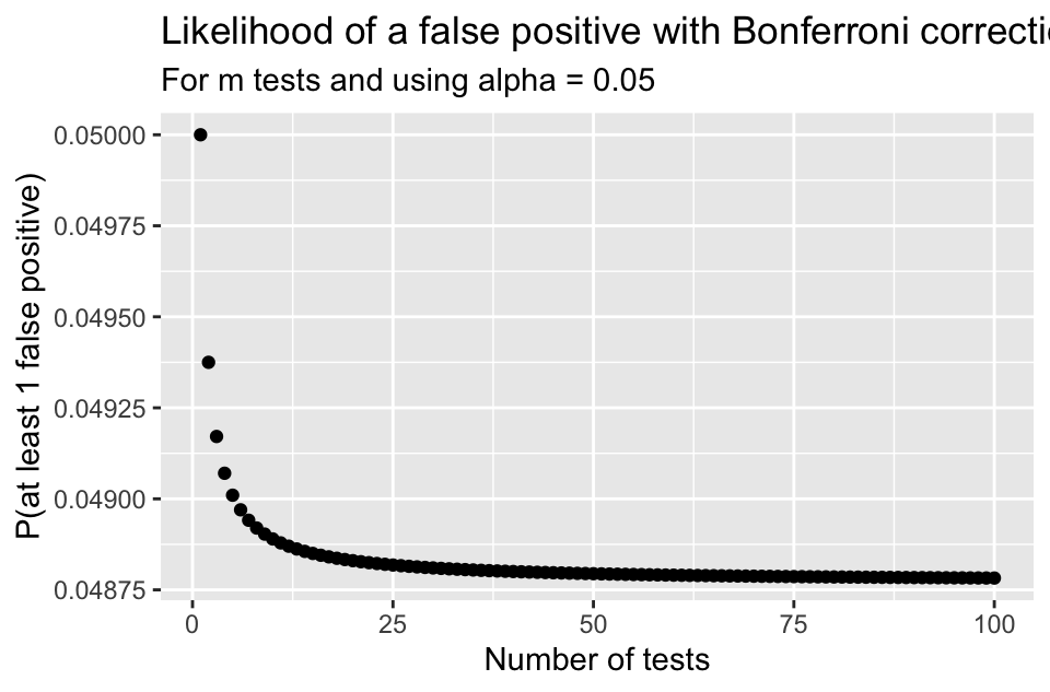
The Bonferroni Correction (1/2)

A very conservative (but very popular) approach is to divide the \(\alpha\) level by how many tests \(m\) are being done:

\[\alpha_{Bonf} = \frac{\alpha}{m}\]

This is equivalent to multiplying the
p-values by m:

\[p\textrm{-value} < \alpha_{Bonf} = \frac{\alpha}{m}\] is the same as \[m \cdot (p\textrm{-value}) < \alpha\] The Bonferroni correction is popular since it’s very easy to implement.

The plot below shows the likelihood of making at least one Type I error depending on how may tests are done.
Notice the likelihood decreases very quickly
- Unfortunately the likelihood of a Type II error is increasing as well
- It becomes “harder” and harder to reject \(H_0\) if doing many tests.

The Bonferroni Correction (2/2)

Pairwise t-tests without any p-value adjustments:

pairwise.t.test(employ$score, 
                employ$disability, 
                p.adj="none")


    Pairwise comparisons using t tests with pooled SD 

data:  employ$score and employ$disability 

           none   amputation crutches hearing
amputation 0.4477 -          -        -      
crutches   0.1028 0.0184     -        -      
hearing    0.1732 0.5418     0.0035   -      
wheelchair 0.4756 0.1433     0.3520   0.0401 

P value adjustment method: none

Pairwise t-tests with Bonferroni p-value adjustments:

pairwise.t.test(employ$score,  
                employ$disability, 
                p.adj="bonferroni")


    Pairwise comparisons using t tests with pooled SD 

data:  employ$score and employ$disability 

           none  amputation crutches hearing
amputation 1.000 -          -        -      
crutches   1.000 0.184      -        -      
hearing    1.000 1.000      0.035    -      
wheelchair 1.000 1.000      1.000    0.401  

P value adjustment method: bonferroni

Since there were 10 tests, all the p-values were multiplied by 10.
Are there any significant pairwise differences?

Tukey’s Honest Significance Test (HSD)

Tukey’s Honest Significance Test (HSD) controls the “family-wise probability” of making a Type I error using a much less conservative method than Bonferroni
- It is specific to ANOVA
In addition to adjusted p-values, it also calculates Tukey adjusted CI’s for all pairwise differences
The function TukeyHSD() creates a set of confidence intervals of the differences between means with the specified family-wise probability of coverage.

# need to run the model using `aov` instead of `lm`
empl_aov <- aov(score ~ disability, data = employ) 

TukeyHSD(x=empl_aov, conf.level = 0.95)

  Tukey multiple comparisons of means
    95% family-wise confidence level

Fit: aov(formula = score ~ disability, data = employ)

$disability
                            diff        lwr        upr     p adj
amputation-none       -0.4714286 -2.2031613  1.2603042 0.9399911
crutches-none          1.0214286 -0.7103042  2.7531613 0.4686233
hearing-none          -0.8500000 -2.5817328  0.8817328 0.6442517
wheelchair-none        0.4428571 -1.2888756  2.1745899 0.9517374
crutches-amputation    1.4928571 -0.2388756  3.2245899 0.1232819
hearing-amputation    -0.3785714 -2.1103042  1.3531613 0.9724743
wheelchair-amputation  0.9142857 -0.8174470  2.6460185 0.5781165
hearing-crutches      -1.8714286 -3.6031613 -0.1396958 0.0277842
wheelchair-crutches   -0.5785714 -2.3103042  1.1531613 0.8812293
wheelchair-hearing     1.2928571 -0.4388756  3.0245899 0.2348141

plot(TukeyHSD(x=empl_aov, conf.level = 0.95))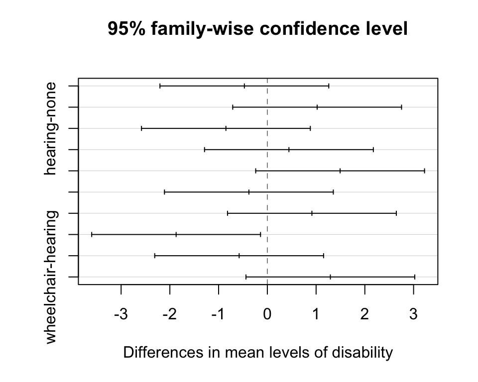

Visualization of pairwise CI’s
Which pair(s) of disabilities are significant after Tukey’s adjustments?

There are many more multiple testing adjustment procedures

Bonferroni is popular because it’s so easy to apply
Tukey’s HSD is usually used for ANOVA
Code below used Holm’s adjustment

# default is Holm's adjustments
pairwise.t.test(employ$score, 
                employ$disability)


    Pairwise comparisons using t tests with pooled SD 

data:  employ$score and employ$disability 

           none  amputation crutches hearing
amputation 1.000 -          -        -      
crutches   0.719 0.165      -        -      
hearing    0.866 1.000      0.035    -      
wheelchair 1.000 0.860      1.000    0.321  

P value adjustment method: holm

False discovery rate (fdr) p-value adjustments are popular in omics, or whenever there are many tests being run:

pairwise.t.test(employ$score, 
                employ$disability, 
                p.adj="fdr")


    Pairwise comparisons using t tests with pooled SD 

data:  employ$score and employ$disability 

           none  amputation crutches hearing
amputation 0.528 -          -        -      
crutches   0.257 0.092      -        -      
hearing    0.289 0.542      0.035    -      
wheelchair 0.528 0.287      0.503    0.134  

P value adjustment method: fdr

Multiple testing

post-hoc testing vs. testing many outcomes

https://xkcd.com/882/

Multiple testing: controlling the Type I error rate

The multiple testing issue is not unique to ANOVA post-hoc testing.
It is also a concern when running separate tests for many related outcomes.
Beware of p-hacking!

Problem:

Although one test has an \(\alpha\) chance of a Type I error (finding a difference between a pair that aren’t different),
the overall Type I error rate will be much higher when running many tests simultaneously.

ANOVA Summary

\[\begin{align} H_0 &: \mu_1 = \mu_2 = ... = \mu_k\\ \text{vs. } H_A&: \text{At least one pair } \mu_i \neq \mu_j \text{ for } i \neq j \end{align}\]

ANOVA table in R:

lm(score ~ disability, data = employ) %>% anova()

Analysis of Variance Table

Response: score
           Df  Sum Sq Mean Sq F value  Pr(>F)  
disability  4  30.521  7.6304  2.8616 0.03013 *
Residuals  65 173.321  2.6665                  
---
Signif. codes:  0 '***' 0.001 '**' 0.01 '*' 0.05 '.' 0.1 ' ' 1

ANOVA table
F-distribution & p-value

Post-hoc testing

Load packages

Goals for today (Section 5.5)

Disability Discrimination Example

Load interview data from .txt file

Factor variable: Make disability variable a factor variable

Factor variable: Change order & name of disability levels

Data viz

ANOVA

Hypotheses

Comparing means

ANOVA in base R

ANOVA tables

ANOVA: Analysis of Variance

Notation

Total Sums of Squares Visually

Calculate Total Sums of Squares

Sums of Squares due to Groups Visually (“between” groups)

Calculate Sums of Squares due to Groups (“between” groups)

Sums of Squares Error Visually (within groups)

Calculate Sums of Squares Error (within groups)

Verify SST = SSG + SSE

Thinking about the F-statistic

ANOVA in base R

Conclusion to hypothesis test

Conditions for ANOVA

Testing variances (Condition 3)

The F-distribution

Which groups are statistically different?

Post-hoc testing for ANOVA

Post-hoc testing: pairwise t-tests

The Bonferroni Correction (1/2)

The Bonferroni Correction (2/2)

Tukey’s Honest Significance Test (HSD)

There are many more multiple testing adjustment procedures

Multiple testing

Multiple testing: controlling the Type I error rate

ANOVA Summary

Load interview data from `.txt` file

Factor variable: Make `disability` variable a factor variable