Code
# run these every time you open Rstudio
library(tidyverse)
library(oibiostat)
library(janitor)
library(rstatix)
library(knitr)
library(gtsummary)
library(moderndive)
library(gt)
library(broom)
library(here)
library(pwr) # new-ishBSTA 511/611
# run these every time you open Rstudio
library(tidyverse)
library(oibiostat)
library(janitor)
library(rstatix)
library(knitr)
library(gtsummary)
library(moderndive)
library(gt)
library(broom)
library(here)
library(pwr) # new-ishAdd text to a plot using annotate():
ggplot(NULL, aes(c(0,4))) +  # no dataset, create axes for x from 0 to 4
  geom_area(stat = "function", fun = dchisq, args = list(df=2),
            fill = "blue", xlim = c(0, 1.0414)) +
  geom_area(stat = "function", fun = dchisq, args = list(df=2),
            fill = "violet", xlim = c(1.0414, 4)) +
  geom_vline(xintercept = 1.0414) +  # vertical line at x = 1.0414
  annotate("text", x = 1.1, y = .4, # add text at specified (x,y) coordinate
           label = "chi-squared = 1.0414", hjust=0, size=6) +
  annotate("text", x = 1.3, y = .1,
label = "p-value = 0.59", hjust=0, size=6) 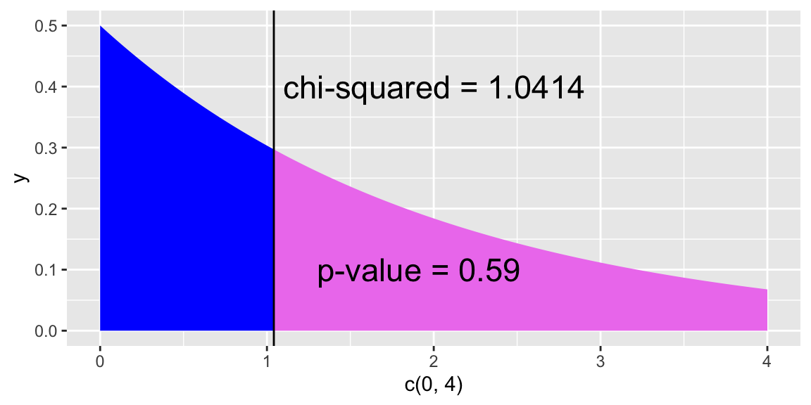
chisq.test()Testing the association (independence) between two categorical variables
NHANES dataset: 10,000 rows, resampled from NHANESraw to undo oversampling effects
Depressed
PhysActive
Generic wording:
Test of “association” wording
\(H_0\): There is no association between the two variables
\(H_A\): There is an association between the two variables
Test of “independence” wording
\(H_0\): The variables are independent
\(H_A\): The variables are not independent
For our example:
Test of “association” wording
\(H_0\): There is no association between depression and physical activity
\(H_A\): There is an association between depression and physical activity
Test of “independence” wording
\(H_0\): The variables depression and physical activity are independent
\(H_A\): The variables depression and physical activity are not independent
Depressed and physically active (PhysActive) variables.See slides for data table.
Below is table in R.
(DepPA_table <- matrix(c(199, 26, 1, 115, 32, 27), nrow = 2, ncol = 3, byrow = T)) [,1] [,2] [,3]
[1,] 199 26 1
[2,] 115 32 27dimnames(DepPA_table) <- list("PA" = c("Yes", "No"), # row names
"Depression" = c("None", "Several", "Most")) # column names
DepPA_table Depression
PA None Several Most
Yes 199 26 1
No 115 32 27\[P(A~and~B)=P(A)P(B)\]
\[\begin{align} P(None~and~Yes) &= P(None)P(Yes)\\ P(None~and~No) &= P(None)P(No)\\ P(Several~and~Yes) &= P(Several)P(Yes)\\ P(Several~and~No) &= P(Several)P(No)\\ P(Most~and~Yes) &= P(Most)P(Yes)\\ P(Most~and~No) &= P(Most)P(No) \end{align}\]
# See slides for data table.
DepPA_table
Depression
PA None Several Most
Yes 199 26 1
No 115 32 27\[\begin{align} P(None~and~Yes) &= \frac{314}{400}\cdot\frac{226}{400}\\ & ...\\ P(Most~and~No) &= \frac{28}{400}\cdot\frac{174}{400} \end{align}\]
With these probabilities, for each cell of the table we calculate the expected counts for each cell under the \(H_0\) hypothesis that the variables are independent
Expected count of Yes & None:
\[\begin{align} 400 \cdot & P(None~and~Yes)\\ &= 400 \cdot P(None)P(Yes)\\ &= 400 \cdot\frac{314}{400}\cdot\frac{226}{400}\\ &= \frac{314\cdot 226}{400} \\ &= 177.41\\ &= \frac{\text{column total}\cdot \text{row total}}{\text{table total}} \end{align}\]
# See slides for data table.
DepPA_table
Depression
PA None Several Most
Yes 199 26 1
No 115 32 27# See slides for data table.
DepPA_table Depression
PA None Several Most
Yes 199 26 1
No 115 32 27See slides for table with expected counts & calculations
Expected count for cell \(i,j\) :
\[\textrm{Expected Count}_{\textrm{row } i,\textrm{ col }j}=\frac{(\textrm{row}~i~ \textrm{total})\cdot(\textrm{column}~j~ \textrm{total})}{\textrm{table total}}\]
Test statistic for a test of association (independence):
\[\chi^2 = \sum_{\textrm{all cells}} \frac{(\textrm{observed} - \text{expected})^2}{\text{expected}}\]
# See slides for data table with expected counts.
DepPA_table
Depression
PA None Several Most
Yes 199 26 1
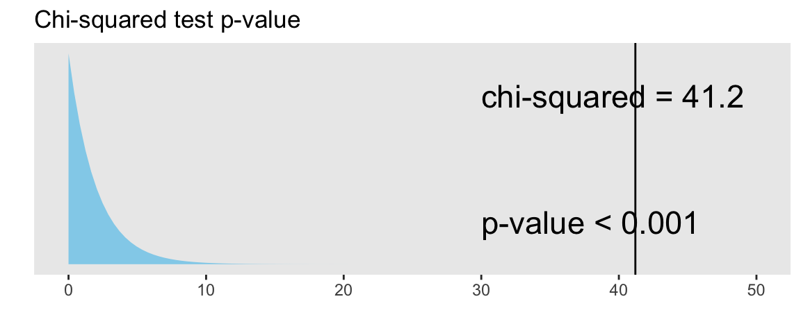
No 115 32 27\[\begin{align} \chi^2 &= \sum\frac{(O-E)^2}{E} \\ &= \frac{(199-177.41)^2}{177.41} + \frac{(26-32.77)^2}{32.77} + \ldots + \frac{(27-12.18)^2}{12.18} \\ &= 41.2 \end{align}\]
Is this value big? Big enough to reject \(H_0\)?
The \(\chi^2\) distribution shape depends on its degrees of freedom
See slides for Chi-squared distribution figure.
pchisq function in R to calculate the probability of being at least as big as the \(\chi^2\) test statistic:pv <- pchisq(41.2, df = 2, lower.tail = FALSE)
pv[1] 1.131185e-09What’s the conclusion to the \(\chi^2\) test?
Recall the hypotheses to our \(\chi^2\) test:
\(H_0\): There is no association between depression and being physically activity
\(H_A\): There is an association between depression and being physically activity
Conclusion:
Based a random sample of 400 US adults from 2009-2012, there is sufficient evidence that there is an association between depression and being physically activity (p-value < 0.001).
If we fail to reject, we DO NOT have evidence of no association.
Create dataset based on results table:
DepPA <- tibble(
  Depression = c(rep("None", 314),
         rep("Several", 58),
         rep("Most", 28)),
  PA = c(rep("Yes", 199),  # None
          rep("No", 115),
          rep("Yes", 26), # Several
          rep("No", 32),
          rep("Yes", 1), # Most
          rep("No", 27))
)
Summary table of data:
DepPA %>% tabyl(Depression, PA) Depression No Yes
Most 27 1
None 115 199
Several 32 26# base R:
table(DepPA) PA
 Depression  No Yes
       Most  27   1
       None 115 199
Several 32 26If only have 2 columns in the dataset:
(ChisqTest_DepPA <-
   chisq.test(table(DepPA)))
    Pearson's Chi-squared test

data:  table(DepPA)
X-squared = 41.171, df = 2, p-value = 1.148e-09
If have >2 columns in the dataset, we need to specify which columns to table:
(ChisqTest_DepPA <-
   chisq.test(table(
     DepPA$Depression, DepPA$PA)))
    Pearson's Chi-squared test

data:  table(DepPA$Depression, DepPA$PA)
X-squared = 41.171, df = 2, p-value = 1.148e-09
The tidyverse way (fewer parentheses)
table(DepPA$Depression, DepPA$PA) %>%
  chisq.test()
    Pearson's Chi-squared test

data:  .
X-squared = 41.171, df = 2, p-value = 1.148e-09
tidy() the output (from broom package):
table(DepPA$Depression, DepPA$PA) %>%
  chisq.test() %>%
tidy() %>% gt()| statistic | p.value | parameter | method |
|---|---|---|---|
| 41.17067 | 1.147897e-09 | 2 | Pearson's Chi-squared test |
Pull p-value
table(DepPA$Depression, DepPA$PA) %>%
  chisq.test() %>%
  tidy() %>% pull(p.value)
[1] 1.147897e-09You can see what the observed and expected counts are from the saved chi-squared test results:
ChisqTest_DepPA$observed
           No Yes
  Most     27   1
  None    115 199
Several 32 26ChisqTest_DepPA$expected
              No    Yes
  Most     12.18  15.82
  None    136.59 177.41
  Several  25.23  32.77
Why is it important to look at the expected counts?
What are we looking for in the expected counts?
Create a base R table of the results:
(DepPA_table <- matrix(c(199, 26, 1, 115, 32, 27), nrow = 2, ncol = 3, byrow = T)) [,1] [,2] [,3]
[1,] 199 26 1
[2,] 115 32 27dimnames(DepPA_table) <- list("PA" = c("Yes", "No"), # row names
"Depression" = c("None", "Several", "Most")) # column names
DepPA_table Depression
PA None Several Most
Yes 199 26 1
No 115 32 27Run \(\chi^2\) test with 2-way table:
chisq.test(DepPA_table)
    Pearson's Chi-squared test

data:  DepPA_table
X-squared = 41.171, df = 2, p-value = 1.148e-09chisq.test(DepPA_table)$expected Depression
PA None Several Most
Yes 177.41 32.77 15.82
No 136.59 25.23 12.18(DepPA_table2x2 <- matrix(c(199, 27, 115, 59), nrow = 2, ncol = 2, byrow = T)) [,1] [,2]
[1,] 199 27
[2,] 115 59dimnames(DepPA_table2x2) <- list("PA" = c("Yes", "No"), # row names
"Depression" = c("None", "Several/Most")) # column names
DepPA_table2x2 Depression
PA None Several/Most
Yes 199 27
No 115 59Output without a CC
chisq.test(DepPA_table2x2, correct = FALSE)
    Pearson's Chi-squared test

data:  DepPA_table2x2
X-squared = 28.093, df = 1, p-value = 1.156e-07
Compare to output with CC:
chisq.test(DepPA_table2x2)
    Pearson's Chi-squared test with Yates' continuity correction

data:  DepPA_table2x2
X-squared = 26.807, df = 1, p-value = 2.248e-07Use this if expected cell counts are too small
(DepPA100_table <- matrix(c(43, 5, 2, 40, 4, 6), nrow = 2, ncol = 3, byrow = T)) [,1] [,2] [,3]
[1,] 43 5 2
[2,] 40 4 6dimnames(DepPA100_table) <- list("PA" = c("Yes", "No"), # row names
"Depression" = c("None", "Several", "Most")) # column names
DepPA100_table Depression
PA None Several Most
Yes 43 5 2
No 40 4 6chisq.test(DepPA100_table) Warning in stats::chisq.test(x, y, ...): Chi-squared approximation may be
incorrect
    Pearson's Chi-squared test

data:  DepPA100_table
X-squared = 2.2195, df = 2, p-value = 0.3296chisq.test(DepPA100_table)$expectedWarning in stats::chisq.test(x, y, ...): Chi-squared approximation may be
incorrect Depression
PA None Several Most
Yes 41.5 4.5 4
No 41.5 4.5 4fisher.test(DepPA100_table)
    Fisher's Exact Test for Count Data

data:  DepPA100_table
p-value = 0.3844
alternative hypothesis: two.sidedFrom the chisq.test help file:
set.seed(567)
chisq.test(DepPA100_table, simulate.p.value = TRUE)
    Pearson's Chi-squared test with simulated p-value (based on 2000
    replicates)

data:  DepPA100_table
X-squared = 2.2195, df = NA, p-value = 0.3893If there are only 2 levels in both of the categorical variables being tested, then the p-value from the \(\chi^2\) test is equal to the p-value from the differences in proportions test.
Example: Previously we tested whether the proportion who had participated in sports betting was the same for college and noncollege young adults:
\[\begin{align} H_0:& ~p_{coll} - p_{noncoll} = 0\\ H_A:& ~p_{coll} - p_{noncoll} \neq 0 \end{align}\]
SportsBet_table <- matrix(
  c(175, 94, 137, 77),
  nrow = 2, ncol = 2, byrow = T)

dimnames(SportsBet_table) <- list(
  "Group" = c("College", "NonCollege"), # row names
  "Bet" = c("No", "Yes"))  # column names

SportsBet_table
Bet
Group No Yes
College 175 94
NonCollege 137 77chisq.test(SportsBet_table) %>% tidy() %>% gt()| statistic | p.value | parameter | method |
|---|---|---|---|
| 0.01987511 | 0.8878864 | 1 | Pearson's Chi-squared test with Yates' continuity correction |
prop.test(SportsBet_table) %>% tidy() %>% gt()| estimate1 | estimate2 | statistic | p.value | parameter | conf.low | conf.high | method | alternative |
|---|---|---|---|---|---|---|---|---|
| 0.6505576 | 0.6401869 | 0.01987511 | 0.8878864 | 1 | -0.07973918 | 0.1004806 | 2-sample test for equality of proportions with continuity correction | two.sided |
2*pnorm(sqrt(0.0199), lower.tail=F) # p-value[1] 0.8878167Running the sports betting example as a chi-squared test is actually an example of a test of homogeneity
In a test of homogeneity, proportions can be compared between many groups
\[\begin{align} H_0:&~ p_1 = p_2 = p_2 = \ldots = p_n\\ H_A:&~ p_i \neq p_j \textrm{for at least one pair of } i, j \end{align}\]
It’s an extension of a two proportions test.
The test statistic & p-value are calculated the same was as a chi-squared test of association (independence)
When we fix the margins (whether row or columns) of one of the “variables” (such as in a cohort or case-control study)