Day 10 Part 2: Inference for mean difference from two-sample dependent/paired data (Section 5.2)

BSTA 511/611

Week 6

Author

Affiliation

Meike Niederhausen, PhD

OHSU-PSU School of Public Health

Published

November 6, 2024

Load packages

Packages need to be loaded every time you restart R or render an Qmd file

# run these every time you open Rstudio
library(tidyverse)    
library(oibiostat)
library(janitor)
library(rstatix)
library(knitr)
library(gtsummary)
library(moderndive)
library(gt)
library(broom) # NEW!!

set.seed(456)

You can check whether a package has been loaded or not
- by looking at the Packages tab and
- seeing whether it has been checked off or not

Day 10 Part 2: Inference for mean difference from two-sample dependent/paired data (Section 5.2)

What we covered in Day 10 Part 1

(4.3, 5.1) Hypothesis testing for mean from one sample

Introduce hypothesis testing using the case of analyzing a mean from one sample (group)

Steps of a hypothesis test:
1. level of significance
2. null ( \(H_0\) ) and alternative ( \(H_A\) ) hypotheses
3. test statistic
4. p-value
5. conclusion

Run a hypothesis test in R
- Load a dataset - need to specify location of dataset
- R projects
- Run a t-test in R
- tidy() the test output using broom package

(4.3.3) Confidence intervals (CIs) vs. hypothesis tests

Goals for today: Part 2 - Class discussion

(5.2) Inference for mean difference from dependent/paired 2 samples

Inference: CIs and hypothesis testing
Exploratory data analysis (EDA) to visualize data
Run paired t-test in R

One-sided CIs

Class discussion

Inference for the mean difference from dependent/paired data is a special case of the inference for the mean from just one sample, that was already covered.
Thus this part will be used for class discussion to practice CIs and hypothesis testing for one mean and apply it in this new setting.
In class I will briefly introduce this topic, explain how it is similar and different from what we already covered, and let you work through the slides and code.

CI’s and hypothesis tests for different scenarios:

\[\text{point estimate} \pm z^*(or~t^*)\cdot SE,~~\text{test stat} = \frac{\text{point estimate}-\text{null value}}{SE}\]

Day	Book	Population parameter	Symbol	Point estimate	Symbol	SE
10	5.1	Pop mean	\(\mu\)	Sample mean	\(\bar{x}\)	\(\frac{s}{\sqrt{n}}\)
10	5.2	Pop mean of paired diff	\(\mu_d\) or \(\delta\)	Sample mean of paired diff	\(\bar{x}_{d}\)	???
11	5.3	Diff in pop means	\(\mu_1-\mu_2\)	Diff in sample means	\(\bar{x}_1 - \bar{x}_2\)
12	8.1	Pop proportion	\(p\)	Sample prop	\(\widehat{p}\)
12	8.2	Diff in pop proportions	\(p_1-p_2\)	Diff in sample proportions	\(\widehat{p}_1-\widehat{p}_2\)

Steps in a Hypothesis Test

Set the level of significance \(\alpha\)
Specify the null ( \(H_0\) ) and alternative ( \(H_A\) ) hypotheses
1. In symbols
2. In words
3. Alternative: one- or two-sided?
Calculate the test statistic.
Calculate the p-value based on the observed test statistic and its sampling distribution
Write a conclusion to the hypothesis test
1. Do we reject or fail to reject \(H_0\)?
2. Write a conclusion in the context of the problem

Examples of paired designs (two samples)

Enroll pairs of identical twins to study a disease
Enroll father & son pairs to study cholesterol levels
Studying pairs of eyes
Enroll people and collect data before & after an intervention (longitudinal data)
Textbook example: Compare maximal speed of competitive swimmers wearing a wetsuit vs. wearing a regular swimsuit
- WIll use these data on homework

Come up with 2 more examples of paired study designs.

Can a vegetarian diet change cholesterol levels?

Scenario:
- 24 non-vegetarian people were enrolled in a study
- They were instructed to adopt a vegetarian diet
- Cholesterol levels were measured before and after the diet
Question: Is there evidence to support that cholesterol levels changed after the vegetarian diet?
How to answer the question?
- First, calculate changes (differences) in cholesterol levels
  - We usually do after - before if the data are longitudinal

Calculate CI for the mean difference \(\delta\):

\[\bar{x}_d \pm t^*\cdot\frac{s_d}{\sqrt{n}}\]

Run a hypothesis test

Hypotheses

\[\begin{align} H_0:& \delta = \delta_0 \\ H_A:& \delta \neq \delta_0 \\ (or&~ <, >) \end{align}\]

Test statistic

\[ t_{\bar{x}_d} = \frac{\bar{x}_d - \delta_0}{\frac{s_d}{\sqrt{n}}} \]

EDA: Explore the cholesterol data

Scenario:
- 24 non-vegetarian people were enrolled in a study
- They were instructed to adopt a vegetarian diet
- Cholesterol levels were measured before and after the diet

chol <- read_csv(here::here("data", "chol213.csv"))
glimpse(chol)

Rows: 24
Columns: 2
$ Before <dbl> 195, 145, 205, 159, 244, 166, 250, 236, 192, 224, 238, 197, 169…
$ After  <dbl> 146, 155, 178, 146, 208, 147, 202, 215, 184, 208, 206, 169, 182…

chol %>% 
  get_summary_stats(type = "common") %>% 
  gt()

variable	n	min	max	median	iqr	mean	sd	se	ci
Before	24	137	250	179	44.5	187.792	33.160	6.769	14.002
After	24	125	215	165	38.0	168.250	26.796	5.470	11.315

Make sure you are able to load the data on your computer!

EDA: Cholesterol levels before and after vegetarian diet

Describe the distributions of the before & after data.

ggplot(chol, aes(x=Before)) +
  geom_density()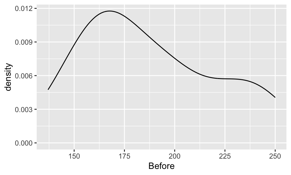

ggplot(chol, aes(x=Before)) +
  geom_boxplot()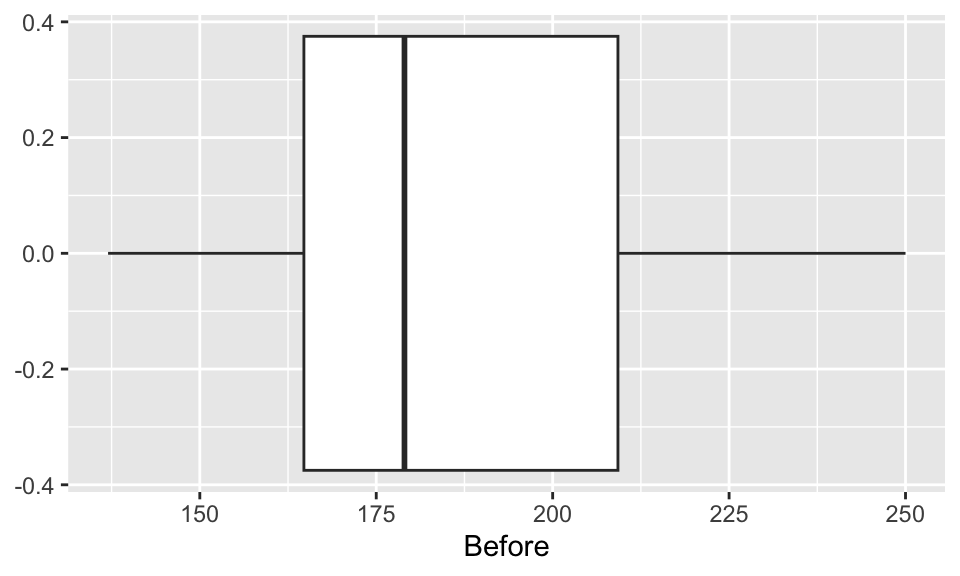

ggplot(chol, aes(x=After)) +
  geom_density()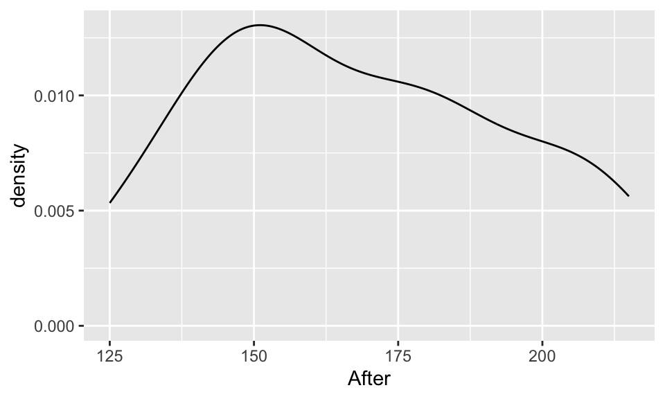

ggplot(chol, aes(x=After)) +
  geom_boxplot()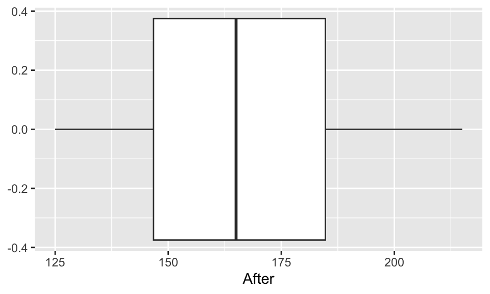

EDA: Spaghetti plot of cholesterol levels before & after diet

Visualize the individual before vs. after diet changes in cholesterol levels

What does this figure tell us?

chol_long <- chol %>% 
  # need an ID column for the plot
  # make it factor so that coloring is not on continuous scale
  mutate(ID = factor(1:n())) %>% 
  # make data long for plot: 
  pivot_longer(
    cols = Before:After,
    names_to = "Time",  # need a column for Before & After on x-axis
    values_to = "Cholesterol") %>% # need a column of all cholesterol values for y-axis
  mutate(
    # change Time a factor variable so that can reorder
    # levels so that Before is before After
    Time = factor(Time, levels = c("Before", "After"))
    )
  
ggplot(chol_long, 
       aes(x=Time, y = Cholesterol, 
           # need to include group = ID 
           # to create a line for each ID
           color = ID, group = ID)) + 
  geom_line(show.legend = FALSE)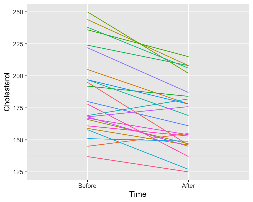

You will not be expected to create this figure yourself.

EDA: Differences in cholesterol levels: After - Before diet

What is this code doing?

chol <- chol %>% 
  mutate(DiffChol = After-Before) 
head(chol, 8)

# A tibble: 8 × 3
  Before After DiffChol
   <dbl> <dbl>    <dbl>
1    195   146      -49
2    145   155       10
3    205   178      -27
4    159   146      -13
5    244   208      -36
6    166   147      -19
7    250   202      -48
8    236   215      -21

Is the mean of DiffChol the same as the difference in means of After - Before? Should it be? Why or why not?

chol %>% 
  get_summary_stats(type = "common") %>% 
  gt()

variable	n	min	max	median	iqr	mean	sd	se	ci
Before	24	137	250	179	44.50	187.792	33.160	6.769	14.002
After	24	125	215	165	38.00	168.250	26.796	5.470	11.315
DiffChol	24	-49	13	-19	20.25	-19.542	16.806	3.430	7.096

EDA: Differences in cholesterol levels: After - Before diet

Compare and contrast the 3 distributions. Comment on shape, center, and spread.

Before & After

ggplot(chol, aes(x=Before)) +
  geom_density()

ggplot(chol, aes(x=After)) +
  geom_density()

DiffChol

ggplot(chol, aes(x=DiffChol)) + 
  geom_density()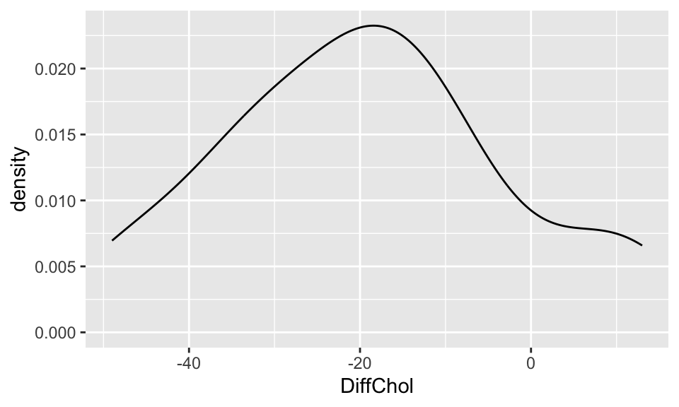

ggplot(chol, aes(x=DiffChol)) + 
  geom_boxplot()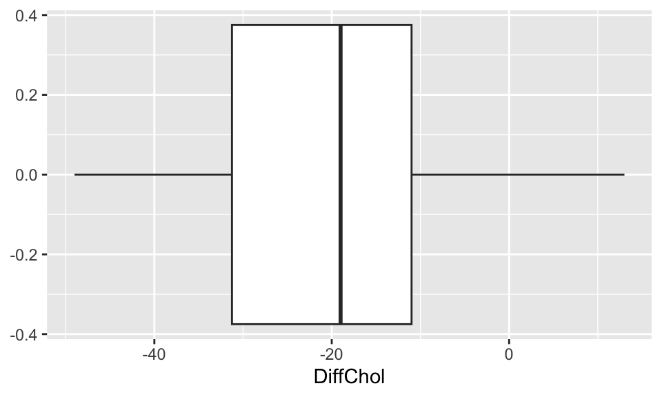

Steps in a Hypothesis Test

Set the level of significance \(\alpha\)
Specify the null ( \(H_0\) ) and alternative ( \(H_A\) ) hypotheses
1. In symbols
2. In words
3. Alternative: one- or two-sided?
Calculate the test statistic.
Calculate the p-value based on the observed test statistic and its sampling distribution
Write a conclusion to the hypothesis test
1. Do we reject or fail to reject \(H_0\)?
2. Write a conclusion in the context of the problem

Step 2: Null & Alternative Hypotheses

Question: Is there evidence to support that cholesterol levels changed after the vegetarian diet?

Null and alternative hypotheses in words Include as much context as possible

\(H_0\): The population mean difference in cholesterol levels after a vegetarian diet is fill in
\(H_A\): The population mean difference in cholesterol levels after a vegetarian diet is fill in

Null and alternative hypotheses in symbols

fill in the missing parts of the hypotheses.

\[~~~~H_0: \delta = \\ H_A: \delta \\\]

Step 3: Test statistic

chol %>% select(DiffChol) %>% get_summary_stats(type = "common") %>% gt()

variable	n	min	max	median	iqr	mean	sd	se	ci
DiffChol	24	-49	13	-19	20.25	-19.542	16.806	3.43	7.096

\[ t_{\bar{x}_d} = \frac{\bar{x}_d - \delta_0}{\frac{s_d}{\sqrt{n}}} \]

Calculate the test statistic.
Based on the value of the test statistic, do you think we are going to reject or fail to reject \(H_0\)?
What probability distribution does the test statistic have?
Are the assumptions for a paired t-test satisfied so that we can use the probability distribution to calculate the \(p\)-value??

n <- 24
alpha <- 0.05
mu <- 0
(p_area <- 1-alpha/2)

[1] 0.975

(xbar <- mean(chol$DiffChol))

[1] -19.54167

(sd <- sd(chol$DiffChol))

[1] 16.80574

(se <- sd/sqrt(n))

[1] 3.430458

(tstat <- (xbar - mu)/se)

[1] -5.696519

Step 4: p-value

The p-value is the probability of obtaining a test statistic just as extreme or more extreme than the observed test statistic assuming the null hypothesis \(H_0\) is true.

# specify upper and lower bounds of shaded region below
mu <- 0
std <- se

# The following figure is only an approximation of the 
# sampling distribution since I used a normal instead
# of t-distribution to make it.

ggplot(data.frame(x = c(mu-6*std, mu+6*std)), aes(x = x)) + 
  stat_function(fun = dnorm, 
                args = list(mean = mu, sd = std)) + 
  scale_y_continuous(breaks = NULL) +
  scale_x_continuous(breaks=c(mu, mu - 3.4*(1:6), mu + 3.4*(1:6))) +
  theme(axis.text.x=element_text(angle = -30, hjust = 0)) +
  labs(y = "", 
       x = "sample mean difference",
       title = "Sampling distribution of mean difference") +
  geom_vline(xintercept = c(-xbar, xbar), 
             color = "red")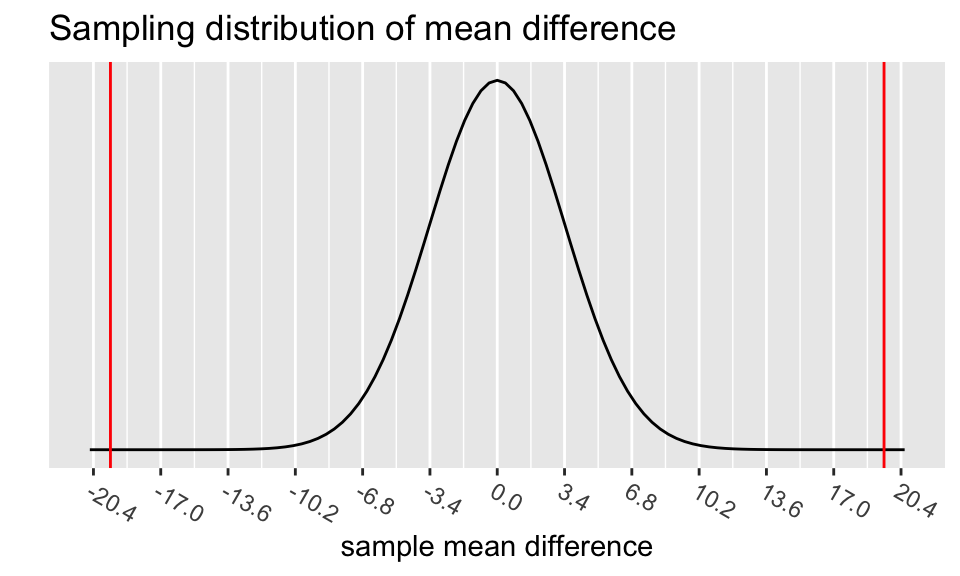

ggplot(data = data.frame(x = c(-6, 6)), aes(x)) + 
  stat_function(fun = dt, args = list(df = n-1)) + 
  ylab("") + 
  xlab("t-dist with df = 23") +
  scale_y_continuous(breaks = NULL) + 
  scale_x_continuous(breaks=c(mu, mu - (1:5), mu + (1:5))) +
  geom_vline(xintercept = c(-tstat,tstat), 
             color = "red")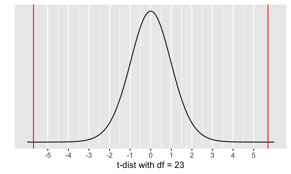

Calculate the p-value and shade in the area representing the p-value:

(pv <- 2*(pt(tstat, df=n-1)))

[1] 8.434775e-06

Step 5: Conclusion to hypothesis test

\[\begin{align} H_0:& \delta = 0 \\ H_A:& \delta \neq 0 \\ \end{align}\]

Recall the \(p\)-value = \(8.434775 \cdot 10 ^{-6}\)
Use \(\alpha\) = 0.05.
Do we reject or fail to reject \(H_0\)?

Conclusion statement:

Stats class conclusion
- There is sufficient evidence that the (population) mean difference in cholesterol levels after a vegetarian diet is different from 0 mg/dL ( \(p\)-value < 0.001).
More realistic manuscript conclusion:
- After a vegetarian diet, cholesterol levels decreased by on average 19.54 mg/dL (SE = 3.43 mg/dL, 2-sided \(p\)-value < 0.001).

95% CI for the mean difference in cholesterol levels

chol %>% select(DiffChol) %>% get_summary_stats(type = "common") %>% gt()

variable	n	min	max	median	iqr	mean	sd	se	ci
DiffChol	24	-49	13	-19	20.25	-19.542	16.806	3.43	7.096

CI for \(\mu_d\) (or \(\delta\)):

n <- 24
alpha <- 0.05
(p_area <- 1-alpha/2)

[1] 0.975

(xbar <- mean(chol$DiffChol))

[1] -19.54167

(sd <- sd(chol$DiffChol))

[1] 16.80574

(tstar <- qt(p_area, df=n-1))  # df = n-1

[1] 2.068658

(se <- sd/sqrt(n))

[1] 3.430458

(moe <- tstar * se)

[1] 7.096443

(LB <- xbar - moe)

[1] -26.63811

(UB <- xbar + moe)

[1] -12.44522

\[\begin{align} \bar{x}_d &\pm t^*\cdot\frac{s_d}{\sqrt{n}}\\ -19.542 &\pm 2.069\cdot\frac{16.806}{\sqrt{24}}\\ -19.542 &\pm 2.069\cdot 3.43\\ -19.542 &\pm 7.096\\ (-26.638&, -12.445) \end{align}\]

Conclusion:
We are 95% that the (population) mean difference in cholesterol levels after a vegetarian diet is between -26.638 mg/dL and -12.445 mg/dL.

Based on the CI, is there evidence the diet made a difference in cholesterol levels? Why or why not?

Running a paired t-test in R

R option 1: Run a 1-sample `t.test` using the paired differences

\(H_A: \delta \neq 0\)

t.test(x = chol$DiffChol, mu = 0)


    One Sample t-test

data:  chol$DiffChol
t = -5.6965, df = 23, p-value = 8.435e-06
alternative hypothesis: true mean is not equal to 0
95 percent confidence interval:
 -26.63811 -12.44522
sample estimates:
mean of x 
-19.54167

Run the code without mu = 0. Do the results change? Why or why not?

R option 2: Run a 2-sample `t.test` with `paired = TRUE` option

\(H_A: \delta \neq 0\)

For a 2-sample t-test we specify both x= and y=
Note: mu = 0 is the default value and doesn’t need to be specified

t.test(x = chol$Before, y = chol$After, mu = 0, paired = TRUE)


    Paired t-test

data:  chol$Before and chol$After
t = 5.6965, df = 23, p-value = 8.435e-06
alternative hypothesis: true mean difference is not equal to 0
95 percent confidence interval:
 12.44522 26.63811
sample estimates:
mean difference 
       19.54167

What is different in the output compared to option 1?

R option 3: Run a 2-sample `t.test` with `paired = TRUE` option, but using the long data and a “formula”

The data have to be in a long format for option 3, where each person has 2 rows: one for Before and one for After.
- The long dataset chol_long was created for the slide “EDA: Spaghetti plot of cholesterol levels before & after diet”.
- See the code to create it there.
What information is being stored in each of the columns?

# first 16 rows of long data:
head(chol_long, 16)

# A tibble: 16 × 3
   ID    Time   Cholesterol
   <fct> <fct>        <dbl>
 1 1     Before         195
 2 1     After          146
 3 2     Before         145
 4 2     After          155
 5 3     Before         205
 6 3     After          178
 7 4     Before         159
 8 4     After          146
 9 5     Before         244
10 5     After          208
11 6     Before         166
12 6     After          147
13 7     Before         250
14 7     After          202
15 8     Before         236
16 8     After          215

Use the usual t.test
What’s different is that
- instead of specifying the variables with x= and y=,
- we give a formula of the form y ~ x using just the variable names,
- and then specify the name of the dataset using data =
This method is often used in practice, and more similar to the coding style of running a regression model (BSTA 512 & 513)

# using long data 
# with columns Cholesterol & Time
t.test(Cholesterol ~ Time, 
       paired = TRUE, 
       data = chol_long)


    Paired t-test

data:  Cholesterol by Time
t = 5.6965, df = 23, p-value = 8.435e-06
alternative hypothesis: true mean difference is not equal to 0
95 percent confidence interval:
 12.44522 26.63811
sample estimates:
mean difference 
       19.54167

What is different in the output compared to option 1?
Rerun the test using Time ~ Cholesterol (switch the variables). What do you get?

Compare the 3 options

How is the code similar and different for the 3 options?
Given a dataset, how would you choose which of the 3 options to use?

# option 1
t.test(x = chol$DiffChol, mu = 0) %>% tidy() %>% gt() # tidy from broom package

estimate	statistic	p.value	parameter	conf.low	conf.high	method	alternative
-19.54167	-5.696519	8.434775e-06	23	-26.63811	-12.44522	One Sample t-test	two.sided

# option 2
t.test(x = chol$Before, y = chol$After, mu = 0, paired = TRUE) %>% tidy() %>% gt()

estimate	statistic	p.value	parameter	conf.low	conf.high	method	alternative
19.54167	5.696519	8.434775e-06	23	12.44522	26.63811	Paired t-test	two.sided

# option 3
t.test(Cholesterol ~ Time, paired = TRUE, data = chol_long) %>% tidy() %>% gt()

estimate	statistic	p.value	parameter	conf.low	conf.high	method	alternative
19.54167	5.696519	8.434775e-06	23	12.44522	26.63811	Paired t-test	two.sided

What if we wanted to test whether the diet decreased cholesterol levels?

What changes in each of the steps?

Set the level of significance \(\alpha\)
Specify the hypotheses \(H_0\) and \(H_A\)
- Alternative: one- or two-sided?
Calculate the test statistic.
Calculate the p-value based on the observed test statistic and its sampling distribution
Write a conclusion to the hypothesis test

R: What if we wanted to test whether the diet decreased cholesterol levels?

Which of the 3 options to run a paired t-test in R is being used below?
How did the code change to account for testing a decrease in cholesterol levels?
Which values in the output changed compared to testing for a change in cholesterol levels? How did they change?

# alternative = c("two.sided", "less", "greater")
t.test(x = chol$DiffChol, mu = 0, alternative = "less") %>% tidy() %>% gt()

estimate	statistic	p.value	parameter	conf.low	conf.high	method	alternative
-19.54167	-5.696519	4.217387e-06	23	-Inf	-13.6623	One Sample t-test	less

One-sided confidence intervals

Formula for a 2-sided (1- \(\alpha\) )% CI:

\[\bar{x} \pm t^*\cdot\frac{s}{\sqrt{n}}\] * \(t^*\) = qt(1-alpha/2, df = n-1) * \(\alpha\) is split over both tails of the distribution

A one-sided (1- \(\alpha\) )% CI has all (1- \(\alpha\) )% on just the left or the right tail of the distribution:

\[(\bar{x} - t^*\cdot\frac{s}{\sqrt{n}},~\infty) \\ (\infty,~\bar{x} + t^*\cdot\frac{s}{\sqrt{n}})\]

\(t^*\) = qt(1-alpha, df = n-1) for a 1-sided lower (1- \(\alpha\) )% CI
\(t^*\) = qt(alpha, df = n-1) for a 1-sided upper (1- \(\alpha\) )% CI
A 1-sided CI gives estimates for a lower or upper bound of the population mean.
See Section 4.2.3 of the V&H book for more

Today & what’s next?

CI’s and hypothesis tests for different scenarios:

\[\text{point estimate} \pm z^*(or~t^*)\cdot SE,~~\text{test stat} = \frac{\text{point estimate}-\text{null value}}{SE}\]

Day	Book	Population parameter	Symbol	Point estimate	Symbol	SE
10	5.1	Pop mean	\(\mu\)	Sample mean	\(\bar{x}\)	\(\frac{s}{\sqrt{n}}\)
10	5.2	Pop mean of paired diff	\(\mu_d\) or \(\delta\)	Sample mean of paired diff	\(\bar{x}_{d}\)	\(\frac{s_d}{\sqrt{n}}\)
11	5.3	Diff in pop means	\(\mu_1-\mu_2\)	Diff in sample means	\(\bar{x}_1 - \bar{x}_2\)	???
12	8.1	Pop proportion	\(p\)	Sample prop	\(\widehat{p}\)
12	8.2	Diff in pop proportions	\(p_1-p_2\)	Diff in sample proportions	\(\widehat{p}_1-\widehat{p}_2\)

Load packages

Day 10 Part 2: Inference for mean difference from two-sample dependent/paired data (Section 5.2)

What we covered in Day 10 Part 1

(4.3, 5.1) Hypothesis testing for mean from one sample

(4.3.3) Confidence intervals (CIs) vs. hypothesis tests

Goals for today: Part 2 - Class discussion

(5.2) Inference for mean difference from dependent/paired 2 samples

One-sided CIs

Class discussion

CI’s and hypothesis tests for different scenarios:

Steps in a Hypothesis Test

Examples of paired designs (two samples)

Can a vegetarian diet change cholesterol levels?

EDA: Explore the cholesterol data

EDA: Cholesterol levels before and after vegetarian diet

EDA: Spaghetti plot of cholesterol levels before & after diet

EDA: Differences in cholesterol levels: After - Before diet

EDA: Differences in cholesterol levels: After - Before diet

Steps in a Hypothesis Test

Step 2: Null & Alternative Hypotheses

Step 3: Test statistic

Step 4: p-value

Step 5: Conclusion to hypothesis test

95% CI for the mean difference in cholesterol levels

Running a paired t-test in R

R option 1: Run a 1-sample t.test using the paired differences

R option 2: Run a 2-sample t.test with paired = TRUE option

R option 3: Run a 2-sample t.test with paired = TRUE option, but using the long data and a “formula”

Compare the 3 options

What if we wanted to test whether the diet decreased cholesterol levels?

R: What if we wanted to test whether the diet decreased cholesterol levels?

One-sided confidence intervals

Today & what’s next?

R option 1: Run a 1-sample `t.test` using the paired differences

R option 2: Run a 2-sample `t.test` with `paired = TRUE` option

R option 3: Run a 2-sample `t.test` with `paired = TRUE` option, but using the long data and a “formula”