# run these every time you open Rstudio
library(tidyverse)
library(oibiostat)
library(ggridges)
library(janitor)
library(rstatix)
library(knitr)
library(gtsummary) # NEW!!Day 3 code: Data visualization
BSTA 511/611 Fall 2024 Day 5, OHSU
Week 3
Load packages
- Packages need to be loaded every time you restart R or render an Qmd file
- You can check whether a package has been loaded or not
- by looking at the Packages tab and
- seeing whether it has been checked off or not
Case study: discrimination in developmental disability support (1.7.1)
In the US, individuals with developmental disabilities typically receive services and support from state governments.
- California allocates funds to developmentally disabled residents through the Department of Developmental Services (DDS)
- Recipients of DDS funds are referred to as “consumers.”
Dataset
dds.discr- sample of 1,000 DDS consumers (out of a total of ~ 250,000)
- data include age, gender, race/ethnicity, and annual DDS financial support per consumer
Previous research
- Researchers examined expenditures on consumers by ethnicity
- Found that the mean annual expenditure on Hispanics was less than that on White non-Hispanics.
Result: an allegation of ethnic discrimination was brought against the California DDS.
Question: Are the data sufficient evidence of ethnic discrimination?
See Section 1.7.1 for more details
Load dds.discr dataset from oibiostat package
The textbook’s datasets are in the R package
oibiostatMake sure the
oibiostatpackage is installed before running the code below.Load the
oibiostatpackage and the datasetdds.discr
the code below needs to be run every time you restart R or render a Qmd file
library(oibiostat)
data("dds.discr")- After loading the dataset
dds.discrusingdata("dds.discr"), you will seedds.discrin the Data list of the Environment window.
Getting to know the dataset
dim(dds.discr)[1] 1000 6names(dds.discr)[1] "id" "age.cohort" "age" "gender" "expenditures"
[6] "ethnicity" length(unique(dds.discr$id)) # How many unique id's are there?[1] 1000str()
- We previously used the base R structure command
str()to get information about variable types in a dataset. - Note this dataset is a
tibbleinstead of adata.frame
str(dds.discr) # base Rtibble [1,000 × 6] (S3: tbl_df/tbl/data.frame)
$ id : int [1:1000] 10210 10409 10486 10538 10568 10690 10711 10778 10820 10823 ...
$ age.cohort : Factor w/ 6 levels "0-5","6-12","13-17",..: 3 5 1 4 3 3 3 3 3 3 ...
$ age : int [1:1000] 17 37 3 19 13 15 13 17 14 13 ...
$ gender : Factor w/ 2 levels "Female","Male": 1 2 2 1 2 1 1 2 1 2 ...
$ expenditures: int [1:1000] 2113 41924 1454 6400 4412 4566 3915 3873 5021 2887 ...
$ ethnicity : Factor w/ 8 levels "American Indian",..: 8 8 4 4 8 4 8 3 8 4 ...
- attr(*, "spec")=
.. cols(
.. ID = col_integer(),
.. `Age Cohort` = col_character(),
.. Age = col_integer(),
.. Gender = col_character(),
.. Expenditures = col_integer(),
.. Ethnicity = col_character()
.. )glimpse()
New: glimpse()
- Use
glimpse()from thetidyversepackage (technically it’s from thedplyrpackage) to get information about variable types. glimpse()tends to have nicer output fortibblesthanstr()
library(tidyverse)
glimpse(dds.discr)  # from tidyverse package (dplyr)
Rows: 1,000
Columns: 6
$ id <int> 10210, 10409, 10486, 10538, 10568, 10690, 10711, 10778, 1…
$ age.cohort <fct> 13-17, 22-50, 0-5, 18-21, 13-17, 13-17, 13-17, 13-17, 13-…
$ age <int> 17, 37, 3, 19, 13, 15, 13, 17, 14, 13, 13, 14, 15, 17, 20…
$ gender <fct> Female, Male, Male, Female, Male, Female, Female, Male, F…
$ expenditures <int> 2113, 41924, 1454, 6400, 4412, 4566, 3915, 3873, 5021, 28…
$ ethnicity <fct> White not Hispanic, White not Hispanic, Hispanic, Hispani…summary()
- We previously used the base R structure command
summary()to get summary information about variables
summary(dds.discr) # base R id age.cohort age gender expenditures
Min. :10210 0-5 : 82 Min. : 0.0 Female:503 Min. : 222
1st Qu.:31809 6-12 :175 1st Qu.:12.0 Male :497 1st Qu.: 2899
Median :55384 13-17:212 Median :18.0 Median : 7026
Mean :54663 18-21:199 Mean :22.8 Mean :18066
3rd Qu.:76135 22-50:226 3rd Qu.:26.0 3rd Qu.:37713
Max. :99898 51+ :106 Max. :95.0 Max. :75098
ethnicity
White not Hispanic:401
Hispanic :376
Asian :129
Black : 59
Multi Race : 26
American Indian : 4
(Other) : 5 Getting to know the dataset: tbl_summary()
- New: Use
tbl_summary()from thegtsummarypackage to get summary information
# library(gtsummary)
tbl_summary(dds.discr)  # from package gtsummary
Characteristic |
N = 1,000 |
|---|---|
| id | 55,385 (31,759, 76,205) |
| age.cohort | |
| 0-5 | 82 (8.2%) |
| 6-12 | 175 (18%) |
| 13-17 | 212 (21%) |
| 18-21 | 199 (20%) |
| 22-50 | 226 (23%) |
| 51+ | 106 (11%) |
| age | 18 (12, 26) |
| gender | |
| Female | 503 (50%) |
| Male | 497 (50%) |
| expenditures | 7,026 (2,898, 37,718) |
| ethnicity | |
| American Indian | 4 (0.4%) |
| Asian | 129 (13%) |
| Black | 59 (5.9%) |
| Hispanic | 376 (38%) |
| Multi Race | 26 (2.6%) |
| Native Hawaiian | 3 (0.3%) |
| Other | 2 (0.2%) |
| White not Hispanic | 401 (40%) |
| 1 Median (Q1, Q3); n (%) |
|
Visualize numerical variables with ggplot
Histograms
What is being measured on the vertical axes?
ggplot(data = dds.discr, aes(x = age)) +
geom_histogram() 
ggplot(data = dds.discr, aes(x = expenditures)) +
geom_histogram() 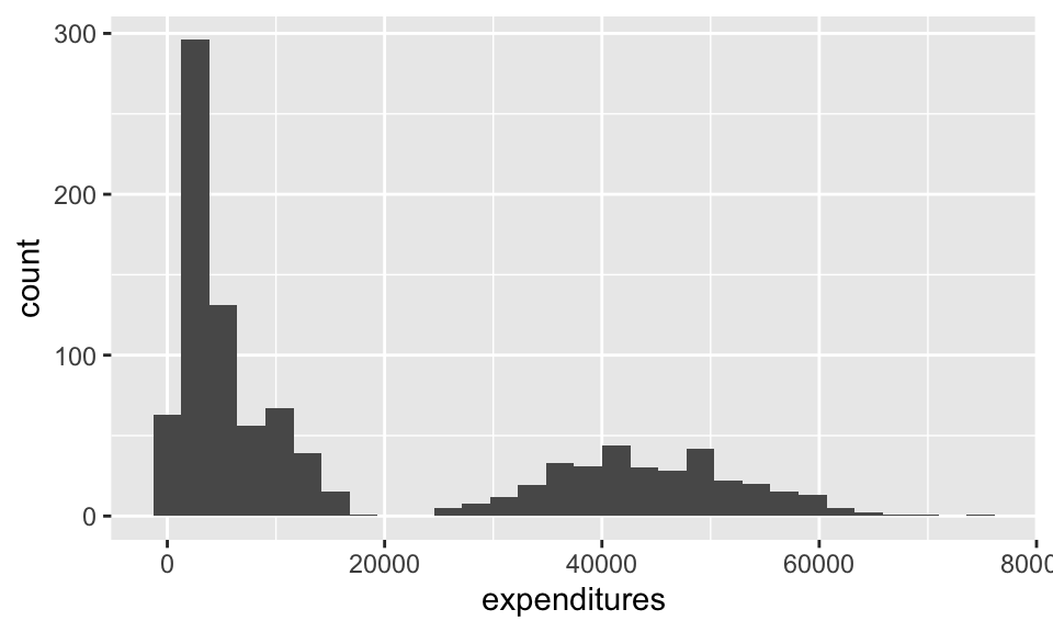
Histograms showing proportions
ggplot(data = dds.discr, aes(x = age)) +
  geom_histogram(aes(y = stat(density)))
Warning: `stat(density)` was deprecated in ggplot2 3.4.0.
ℹ Please use `after_stat(density)` instead.
ggplot(data = dds.discr, aes(x = age)) +
  geom_histogram(aes(y = stat(density))) +
scale_y_continuous(labels = scales::percent_format()) 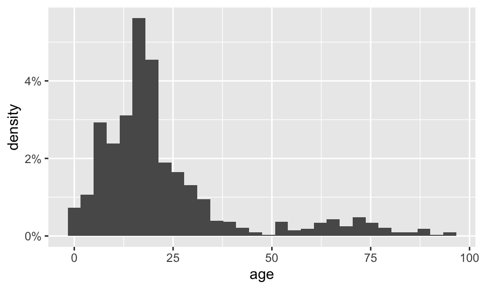
Density plots
What is being measured on the vertical axes?
ggplot(data = dds.discr, aes(x = age)) +
geom_density() 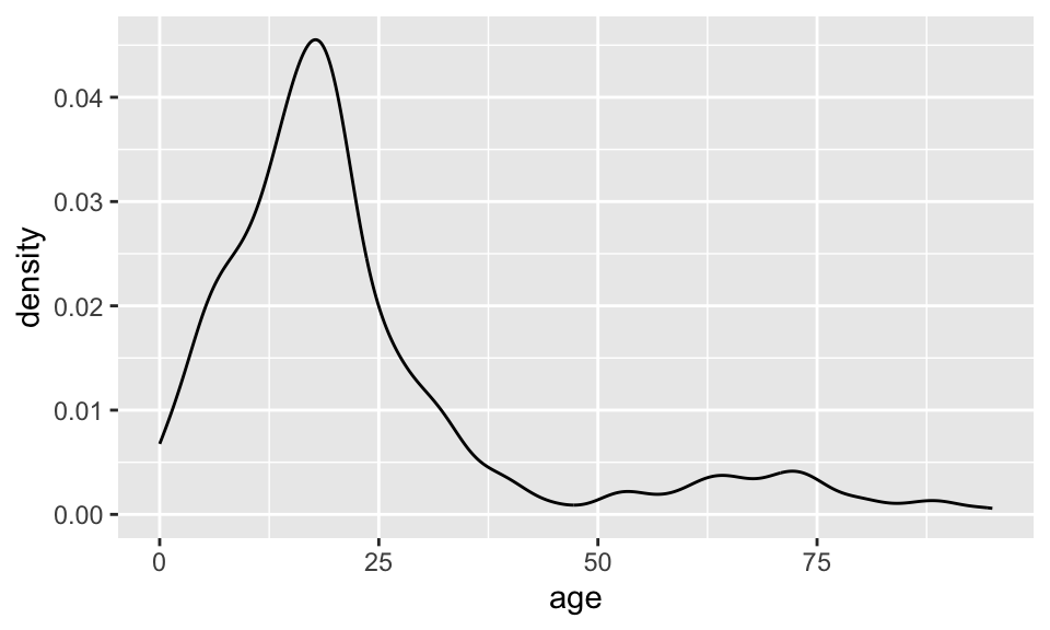
ggplot(data = dds.discr, aes(x = age)) +
geom_histogram() 
Dot plots (better for smaller samples)
What is being measured on the vertical axes?
ggplot(data = dds.discr, aes(x = age)) +
geom_dotplot(binwidth =1) 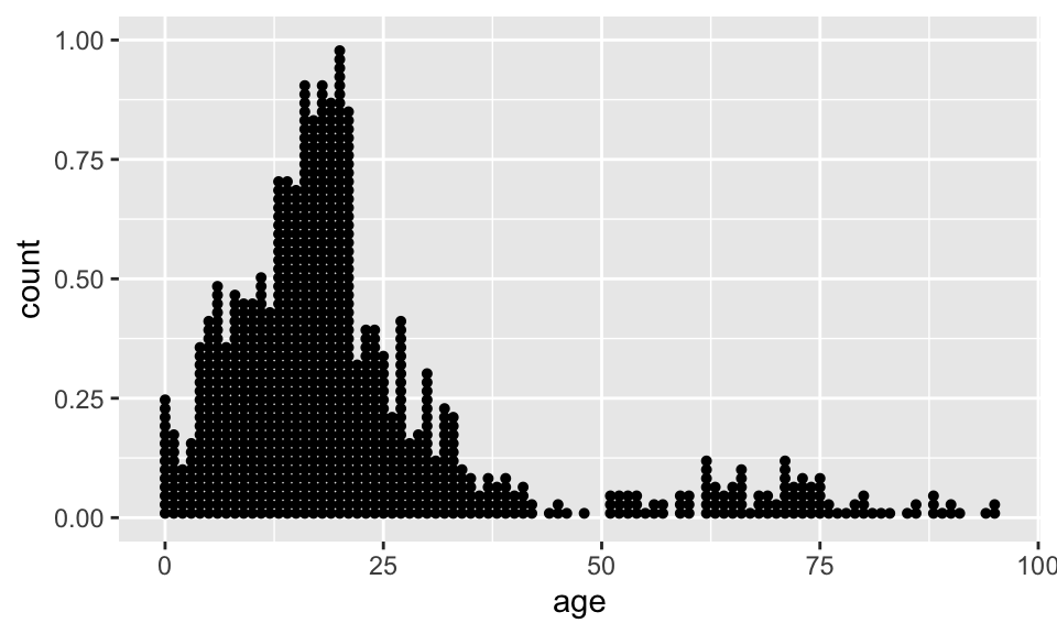
ggplot(data = dds.discr, aes(x = age)) +
geom_histogram(binwidth =1) 
Boxplots
ggplot(data = dds.discr, aes(x = age)) +
geom_boxplot() 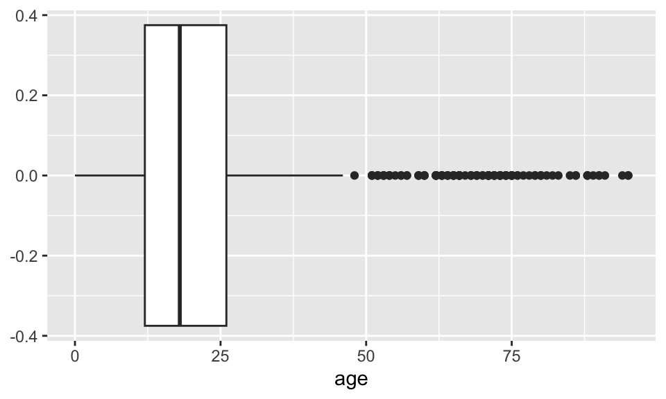
ggplot(data = dds.discr, aes(y = age)) +
geom_boxplot() 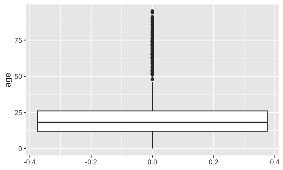
Visualizing relationships between numerical and categorical variables (1.6.3)
Side-by-side boxplots
ggplot(data = dds.discr,
       aes(x = expenditures, y = ethnicity)) +
  geom_boxplot() +
  labs(x = "Annual Expenditures ($)",
y = "Race and ethnicity") 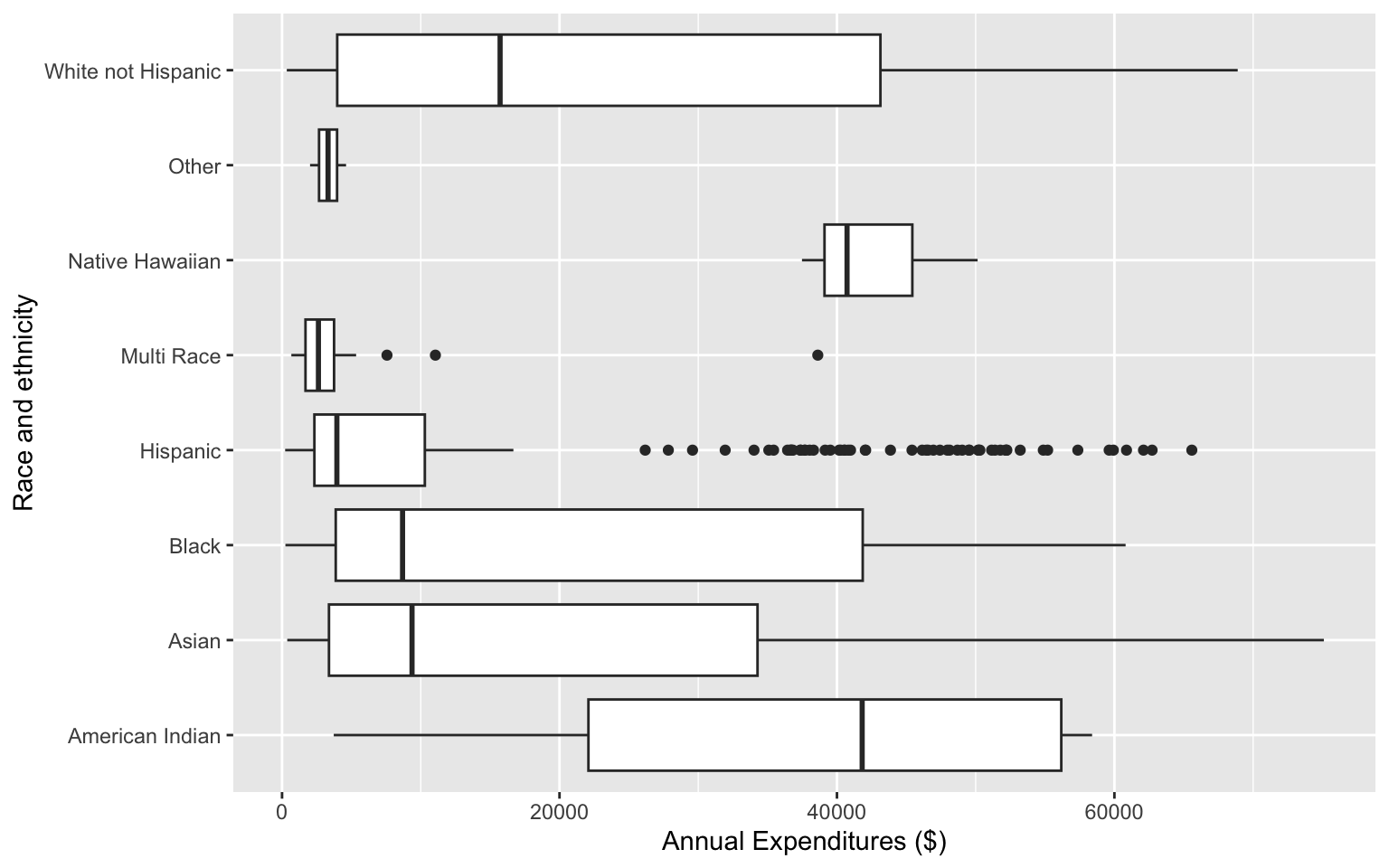
Can you determine the following using boxplots?
- distribution shape
- sample size
Side-by-side boxplots with data points
ggplot(data = dds.discr,
       aes(x = expenditures, y = ethnicity)) +
  geom_boxplot(color="darkgrey") +
  labs(x = "Annual Expenditures ($)",
       y = "Race and ethnicity") +
  geom_jitter(aes(color = ethnicity),
              alpha = 0.3,
              show.legend = FALSE,
              position = position_jitter(height = 0.4)
) 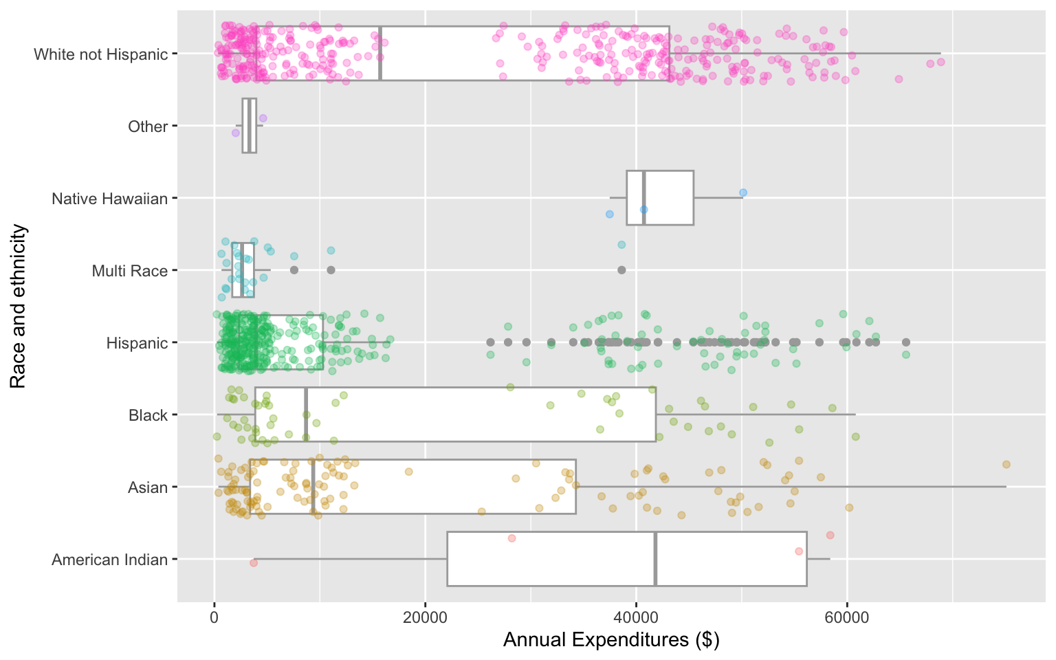
Can you determine the following using boxplots?
- distribution shape
- sample size
Density plots by group
ggplot(data = dds.discr,
       aes(x = expenditures,
           color = ethnicity)) +
  geom_density() +
labs(x = "Annual Expenditures ($)") 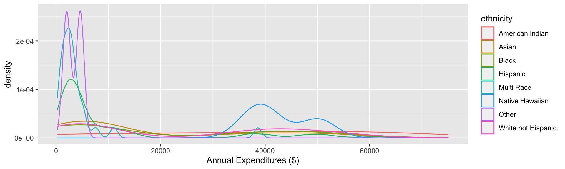
Ridgeline plot
# library(ggridges)
ggplot(data = dds.discr,
       aes(x = expenditures, y = ethnicity,
           fill = ethnicity)) +
  geom_density_ridges(
    alpha = 0.3,
    show.legend = FALSE) +
  labs(x = "Annual Expenditures ($)",
       y = "Race and ethnicity",
title = "Expenditures by race and ethnicity") 
Transforming data (1.4.5)
- We sometimes apply a transformation to highly skewed data to make it more symmetric
- Log transformations are often used for skewed right data
x = expenditures
ggplot(data = dds.discr,
       aes(x = expenditures)) +
geom_density() 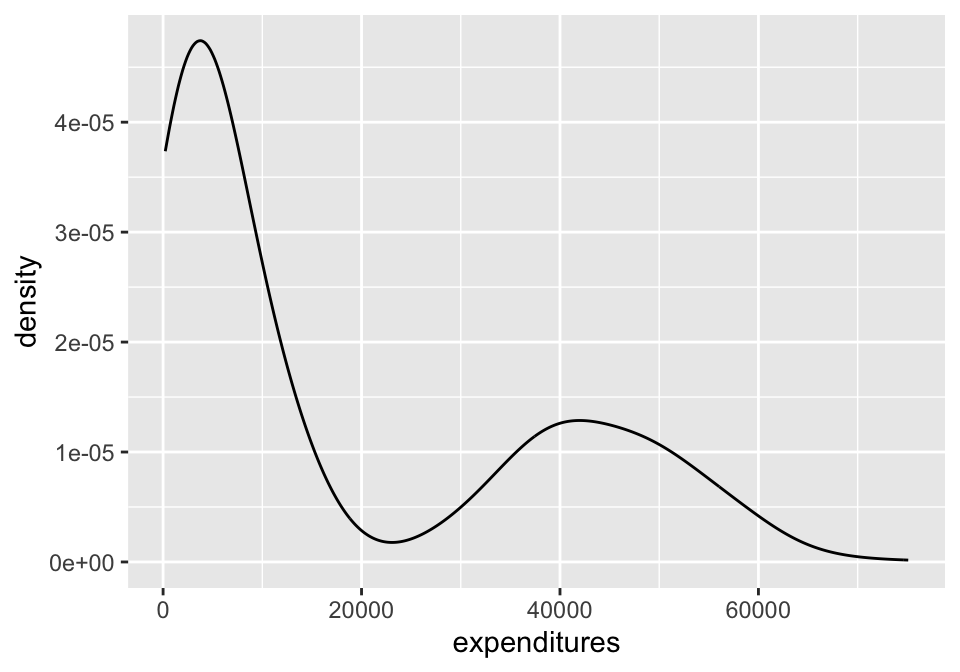
x = log(expenditures)
ggplot(data = dds.discr,
       aes(x = log(expenditures))) +
geom_density() 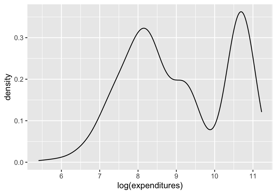
Relationships between two numerical variables (1.6.1)
Scatterplots
ggplot(data = dds.discr,
       aes(x = age, y = expenditures)) +
  geom_point() +
  labs(x = "Age",
y = "Annual Expenditures ($)") 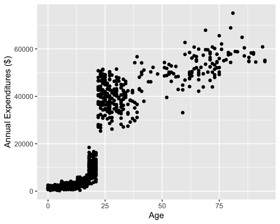
Response vs. explanatory variables (Section 1.2.3) - A response variable measures the outcome of interest in a study - A study will typically examine whether the values of a response variable differ as values of an explanatory variable change
Describe the association between the variables
(Pearson) Correlation coefficient \(r\)
The (Peasron) correlation coefficient of variables \(x\) and \(y\) can be computed using the formula \[r = \frac{1}{n-1}\sum_{i=1}^{n}\Big(\frac{x_i - \bar{x}}{s_x}\Big)\Big(\frac{y_i - \bar{y}}{s_y}\Big)\] where * \((x_1,y_1),(x_2,y_2),...,(x_n,y_n)\) are the \(n\) paired values of the variables \(x\) and \(y\) * \(s_x\) and \(s_y\) are the sample standard deviations of the variables \(x\) and \(y\), respectively
cor(dds.discr$age, dds.discr$expenditures)[1] 0.8432422Scatterplots with color-coded dots
ggplot(data = dds.discr,
       aes(x = age, y = expenditures,
           color = ethnicity)) +
  geom_point(alpha = .5) +
  labs(x = "Age",
y = "Annual Expenditures ($)") 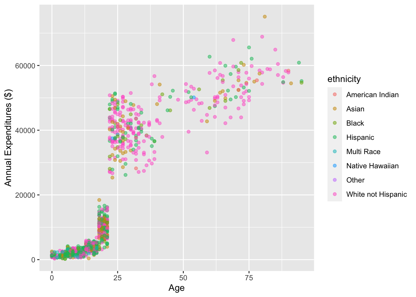
Categorical data (1.5) and Relationships between two categorical variables (1.6.2)
Barplots
Counts
ggplot(data = dds.discr,
       aes(x = ethnicity)) +
geom_bar() 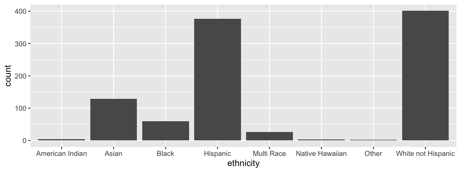
percentages
ggplot(data = dds.discr,
       aes(x = ethnicity)) +
  geom_bar(aes(y = stat(prop), group = 1)) +
scale_y_continuous(labels = scales::percent_format()) 
Barplots with 2 variables: segmented bar plots
ggplot(data = dds.discr,
       aes(x = ethnicity,
           fill = age.cohort)) +
geom_bar() 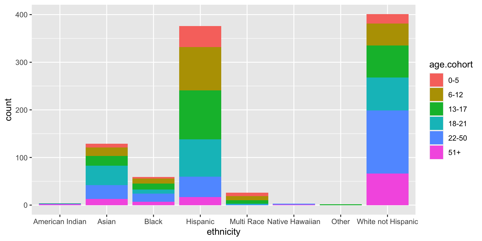
ggplot(data = dds.discr,
       aes(x = ethnicity,
           fill = age.cohort)) +
geom_bar(position = "fill") 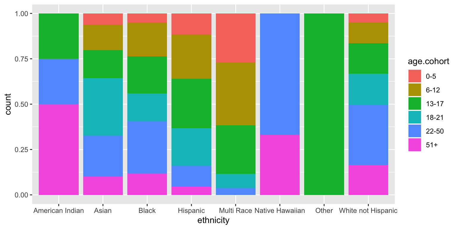
Barplots with 2 variables: side-by-side bar plots
Side-by-side bar plot
ggplot(data = dds.discr,
       aes(x = ethnicity,
           fill = age.cohort)) +
geom_bar(position = "dodge") 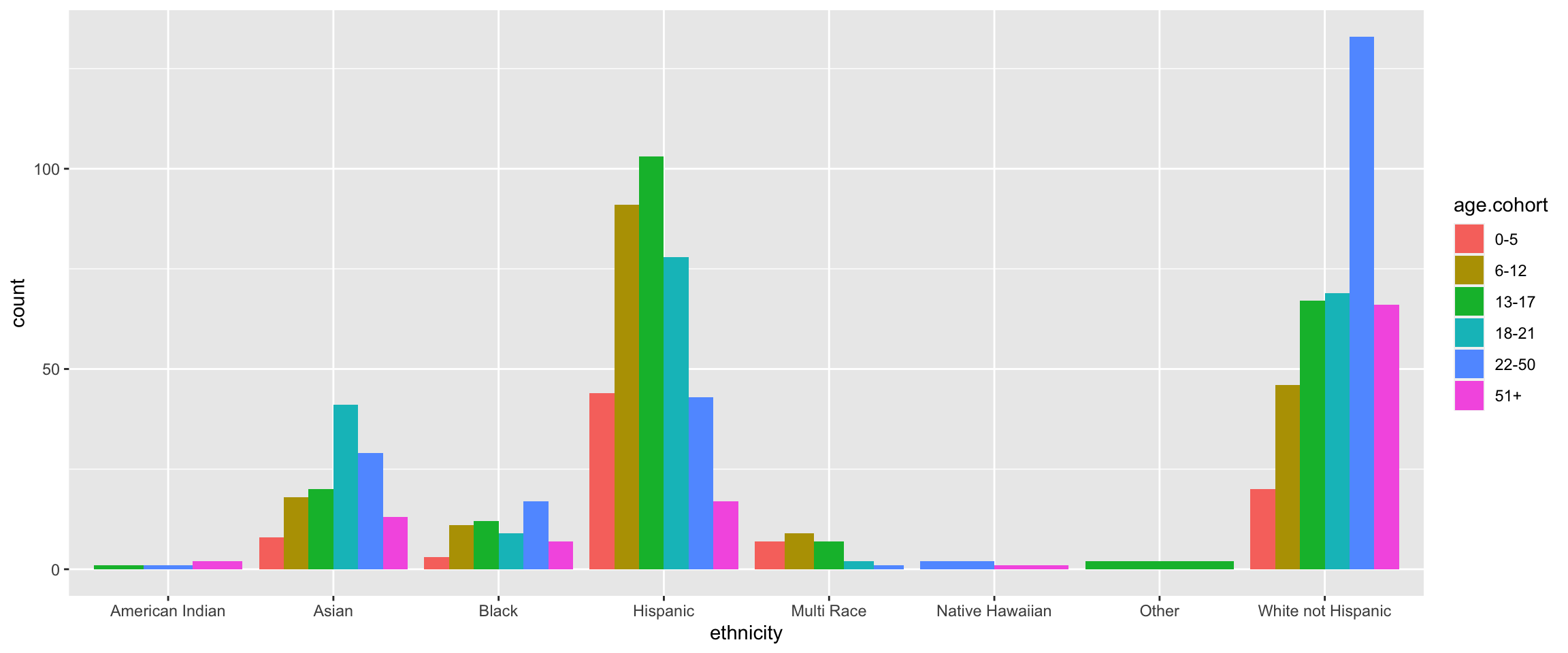
Summarizing categorical data and some data wrangling
Frequency tables: count()
countis from thedplyrpackage- the output is a long tibble, and not a “nice” table
dds.discr %>% count(ethnicity)# A tibble: 8 × 2
ethnicity n
<fct> <int>
1 American Indian 4
2 Asian 129
3 Black 59
4 Hispanic 376
5 Multi Race 26
6 Native Hawaiian 3
7 Other 2
8 White not Hispanic 401dds.discr %>%
count(ethnicity, age.cohort)# A tibble: 35 × 3
ethnicity age.cohort n
<fct> <fct> <int>
1 American Indian 13-17 1
2 American Indian 22-50 1
3 American Indian 51+ 2
4 Asian 0-5 8
5 Asian 6-12 18
6 Asian 13-17 20
7 Asian 18-21 41
8 Asian 22-50 29
9 Asian 51+ 13
10 Black 0-5 3
# ℹ 25 more rowsHow to use the pipe %>%
The pipe operator %>% strings together commands to be performed sequentially
dds.discr %>% head(n=3) # pronounce %>% as "then"# A tibble: 3 × 6
id age.cohort age gender expenditures ethnicity
<int> <fct> <int> <fct> <int> <fct>
1 10210 13-17 17 Female 2113 White not Hispanic
2 10409 22-50 37 Male 41924 White not Hispanic
3 10486 0-5 3 Male 1454 Hispanic - Always first list the tibble that the commands are being applied to
- Can use multiple pipes to run multiple commands in sequence
- What does the following code do?
dds.discr %>% head(n=3) %>% summary() id age.cohort age gender expenditures
Min. :10210 0-5 :1 Min. : 3 Female:1 Min. : 1454
1st Qu.:10310 6-12 :0 1st Qu.:10 Male :2 1st Qu.: 1784
Median :10409 13-17:1 Median :17 Median : 2113
Mean :10368 18-21:0 Mean :19 Mean :15164
3rd Qu.:10448 22-50:1 3rd Qu.:27 3rd Qu.:22018
Max. :10486 51+ :0 Max. :37 Max. :41924
ethnicity
White not Hispanic:2
Hispanic :1
American Indian :0
Asian :0
Black :0
Multi Race :0
(Other) :0 Frequency tables: janitor package’s tabyl function
# default table
dds.discr %>%
  tabyl(ethnicity)
ethnicity n percent
American Indian 4 0.004
Asian 129 0.129
Black 59 0.059
Hispanic 376 0.376
Multi Race 26 0.026
Native Hawaiian 3 0.003
Other 2 0.002
White not Hispanic 401 0.401adorn_ your table!
dds.discr %>%
  tabyl(ethnicity) %>%
  adorn_totals("row") %>%
  adorn_pct_formatting(digits=2)
ethnicity n percent
American Indian 4 0.40%
Asian 129 12.90%
Black 59 5.90%
Hispanic 376 37.60%
Multi Race 26 2.60%
Native Hawaiian 3 0.30%
Other 2 0.20%
White not Hispanic 401 40.10%
Total 1000 100.00%Relative frequency table
A relative frequency table shows proportions (or percentages) instead of counts
Below I removed (deselected) the counts column (
n) to create a relative frequency table
dds.discr %>%
  tabyl(ethnicity) %>%
  adorn_totals("row") %>%
  adorn_pct_formatting(digits=2) %>%
  select(-n) # remove column with variable name n
ethnicity percent
American Indian 0.40%
Asian 12.90%
Black 5.90%
Hispanic 37.60%
Multi Race 2.60%
Native Hawaiian 0.30%
Other 0.20%
White not Hispanic 40.10%
Total 100.00%Contingency tables (two-way tables)
- Contingency tables summarize data for two categorical variables
- with each value in the table representing the number of times
a particular combination of outcomes occurs
- with each value in the table representing the number of times
- Row & column totals
are sometimes called marginal totals
dds.discr %>%
  tabyl(ethnicity, gender) %>%
  adorn_totals(c("row", "col"))
ethnicity Female Male Total
American Indian 3 1 4
Asian 61 68 129
Black 26 33 59
Hispanic 192 184 376
Multi Race 13 13 26
Native Hawaiian 2 1 3
Other 1 1 2
White not Hispanic 205 196 401
Total 503 497 1000Contingency tables with percentages
dds.discr %>%
  tabyl(ethnicity, age.cohort) %>%
  adorn_totals(c("row")) %>%
  adorn_percentages("row") %>%
  adorn_pct_formatting(digits=0) %>%
  adorn_ns()
ethnicity 0-5 6-12 13-17 18-21 22-50 51+
American Indian 0% (0) 0% (0) 25% (1) 0% (0) 25% (1) 50% (2)
Asian 6% (8) 14% (18) 16% (20) 32% (41) 22% (29) 10% (13)
Black 5% (3) 19% (11) 20% (12) 15% (9) 29% (17) 12% (7)
Hispanic 12% (44) 24% (91) 27% (103) 21% (78) 11% (43) 5% (17)
Multi Race 27% (7) 35% (9) 27% (7) 8% (2) 4% (1) 0% (0)
Native Hawaiian 0% (0) 0% (0) 0% (0) 0% (0) 67% (2) 33% (1)
Other 0% (0) 0% (0) 100% (2) 0% (0) 0% (0) 0% (0)
White not Hispanic 5% (20) 11% (46) 17% (67) 17% (69) 33% (133) 16% (66)
Total 8% (82) 18% (175) 21% (212) 20% (199) 23% (226) 11% (106)Summarizing numeric data
Mean annual DDS expenditures by race/ethnicity
mean(dds.discr$expenditures)[1] 18065.79dds.discr %>%
summarize(
ave = mean(expenditures),
SD = sd(expenditures),
med = median(expenditures))# A tibble: 1 × 3
ave SD med
<dbl> <dbl> <dbl>
1 18066. 19543. 7026dds.discr %>%
group_by(ethnicity) %>%
summarize(
ave = mean(expenditures),
SD = sd(expenditures),
med = median(expenditures))# A tibble: 8 × 4
ethnicity ave SD med
<fct> <dbl> <dbl> <dbl>
1 American Indian 36438. 25694. 41818.
2 Asian 18392. 19209. 9369
3 Black 20885. 20549. 8687
4 Hispanic 11066. 15630. 3952
5 Multi Race 4457. 7332. 2622
6 Native Hawaiian 42782. 6576. 40727
7 Other 3316. 1836. 3316.
8 White not Hispanic 24698. 20604. 15718 get_summary_stats() from rstatix package
dds.discr %>% get_summary_stats()# A tibble: 3 × 13
variable n min max median q1 q3 iqr mad mean sd
<fct> <dbl> <dbl> <dbl> <dbl> <dbl> <dbl> <dbl> <dbl> <dbl> <dbl>
1 id 1000 10210 99898 55384. 31809. 76135. 44326 3.27e4 5.47e4 2.56e4
2 age 1000 0 95 18 12 26 14 1.04e1 2.28e1 1.85e1
3 expenditures 1000 222 75098 7026 2899. 37713. 34814 7.76e3 1.81e4 1.95e4
# ℹ 2 more variables: se <dbl>, ci <dbl>dds.discr %>%
group_by(ethnicity) %>%
get_summary_stats(expenditures, type = "common")# A tibble: 8 × 11
ethnicity variable n min max median iqr mean sd se ci
<fct> <fct> <dbl> <dbl> <dbl> <dbl> <dbl> <dbl> <dbl> <dbl> <dbl>
1 American… expendi… 4 3726 58392 41818. 34085. 36438. 25694. 12847. 40885.
2 Asian expendi… 129 374 75098 9369 30892 18392. 19209. 1691. 3346.
3 Black expendi… 59 240 60808 8687 37987 20885. 20549. 2675. 5355.
4 Hispanic expendi… 376 222 65581 3952 7961. 11066. 15630. 806. 1585.
5 Multi Ra… expendi… 26 669 38619 2622 2060. 4457. 7332. 1438. 2962.
6 Native H… expendi… 3 37479 50141 40727 6331 42782. 6576. 3797. 16337.
7 Other expendi… 2 2018 4615 3316. 1298. 3316. 1836. 1298. 16499.
8 White no… expendi… 401 340 68890 15718 39157 24698. 20604. 1029. 2023.How to force all output to be shown?
Use kable() from the knitr package.
dds.discr %>% get_summary_stats() %>% kable()| variable | n | min | max | median | q1 | q3 | iqr | mad | mean | sd | se | ci |
|---|---|---|---|---|---|---|---|---|---|---|---|---|
| id | 1000 | 10210 | 99898 | 55384.5 | 31808.75 | 76134.75 | 44326 | 32734.325 | 54662.85 | 25643.673 | 810.924 | 1591.310 |
| age | 1000 | 0 | 95 | 18.0 | 12.00 | 26.00 | 14 | 10.378 | 22.80 | 18.462 | 0.584 | 1.146 |
| expenditures | 1000 | 222 | 75098 | 7026.0 | 2898.75 | 37712.75 | 34814 | 7760.670 | 18065.79 | 19542.831 | 617.999 | 1212.724 |
dds.discr %>%
  group_by(ethnicity) %>%
get_summary_stats(expenditures, type = "common") %>%
kable()| ethnicity | variable | n | min | max | median | iqr | mean | sd | se | ci |
|---|---|---|---|---|---|---|---|---|---|---|
| American Indian | expenditures | 4 | 3726 | 58392 | 41817.5 | 34085.25 | 36438.250 | 25693.912 | 12846.956 | 40884.748 |
| Asian | expenditures | 129 | 374 | 75098 | 9369.0 | 30892.00 | 18392.372 | 19209.225 | 1691.278 | 3346.482 |
| Black | expenditures | 59 | 240 | 60808 | 8687.0 | 37987.00 | 20884.593 | 20549.274 | 2675.288 | 5355.170 |
| Hispanic | expenditures | 376 | 222 | 65581 | 3952.0 | 7961.25 | 11065.569 | 15629.847 | 806.048 | 1584.940 |
| Multi Race | expenditures | 26 | 669 | 38619 | 2622.0 | 2059.75 | 4456.731 | 7332.135 | 1437.950 | 2961.514 |
| Native Hawaiian | expenditures | 3 | 37479 | 50141 | 40727.0 | 6331.00 | 42782.333 | 6576.462 | 3796.922 | 16336.838 |
| Other | expenditures | 2 | 2018 | 4615 | 3316.5 | 1298.50 | 3316.500 | 1836.356 | 1298.500 | 16499.007 |
| White not Hispanic | expenditures | 401 | 340 | 68890 | 15718.0 | 39157.00 | 24697.549 | 20604.376 | 1028.933 | 2022.793 |
Back to research question
Case study: discrimination in developmental disability support (1.7.1)
- Previous research
- Researchers examined DDS expenditures for developmentally disabled residents by ethnicity
- Found that the mean annual expenditures on Hispanics was less than that on White non-Hispanics.
- Result: an allegation of ethnic discrimination was brought against the California DDS.
- Question: Are the data sufficient evidence of ethnic discrimination?