Day 16: Simple Linear Regression Part 2 (Sections 6.3-6.4)
BSTA 511/611
2024-12-02
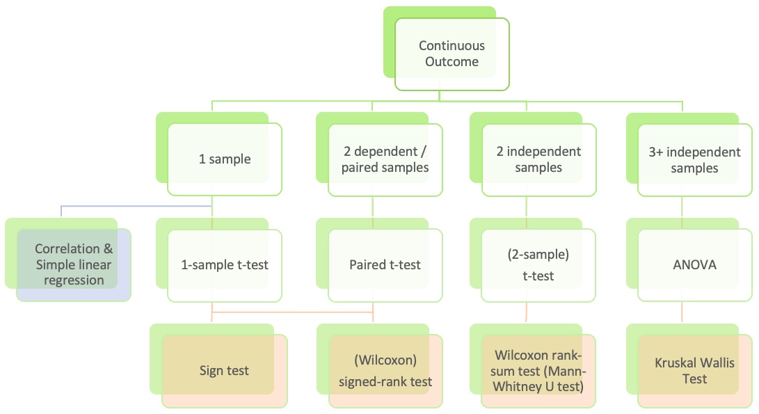
Where are we?
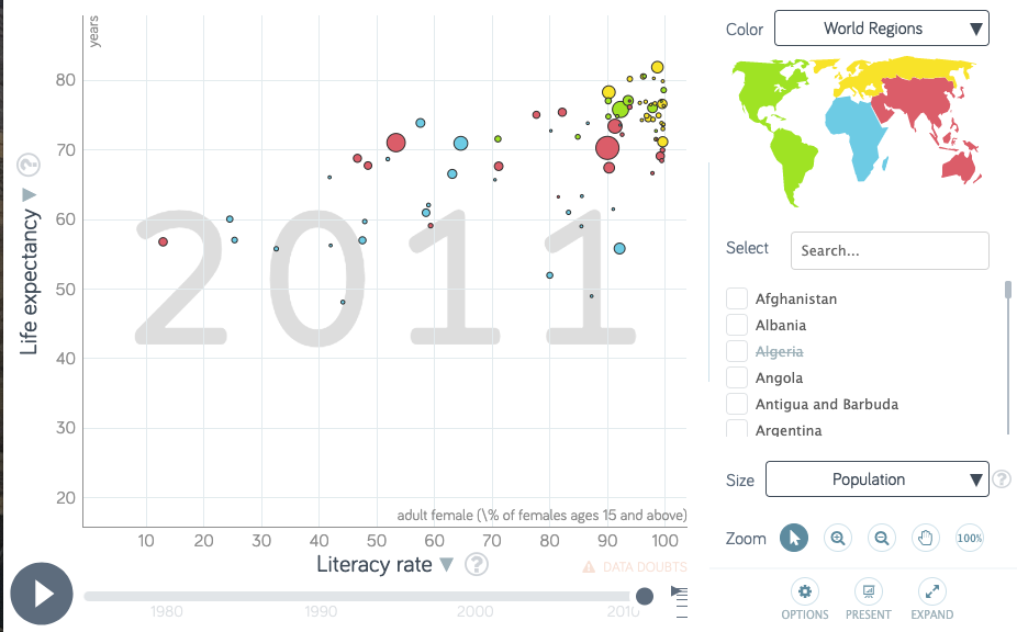
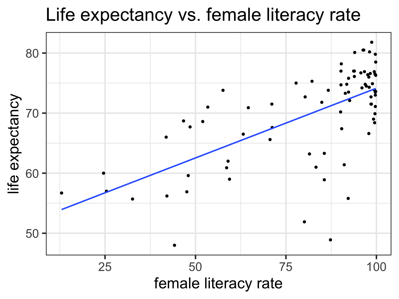
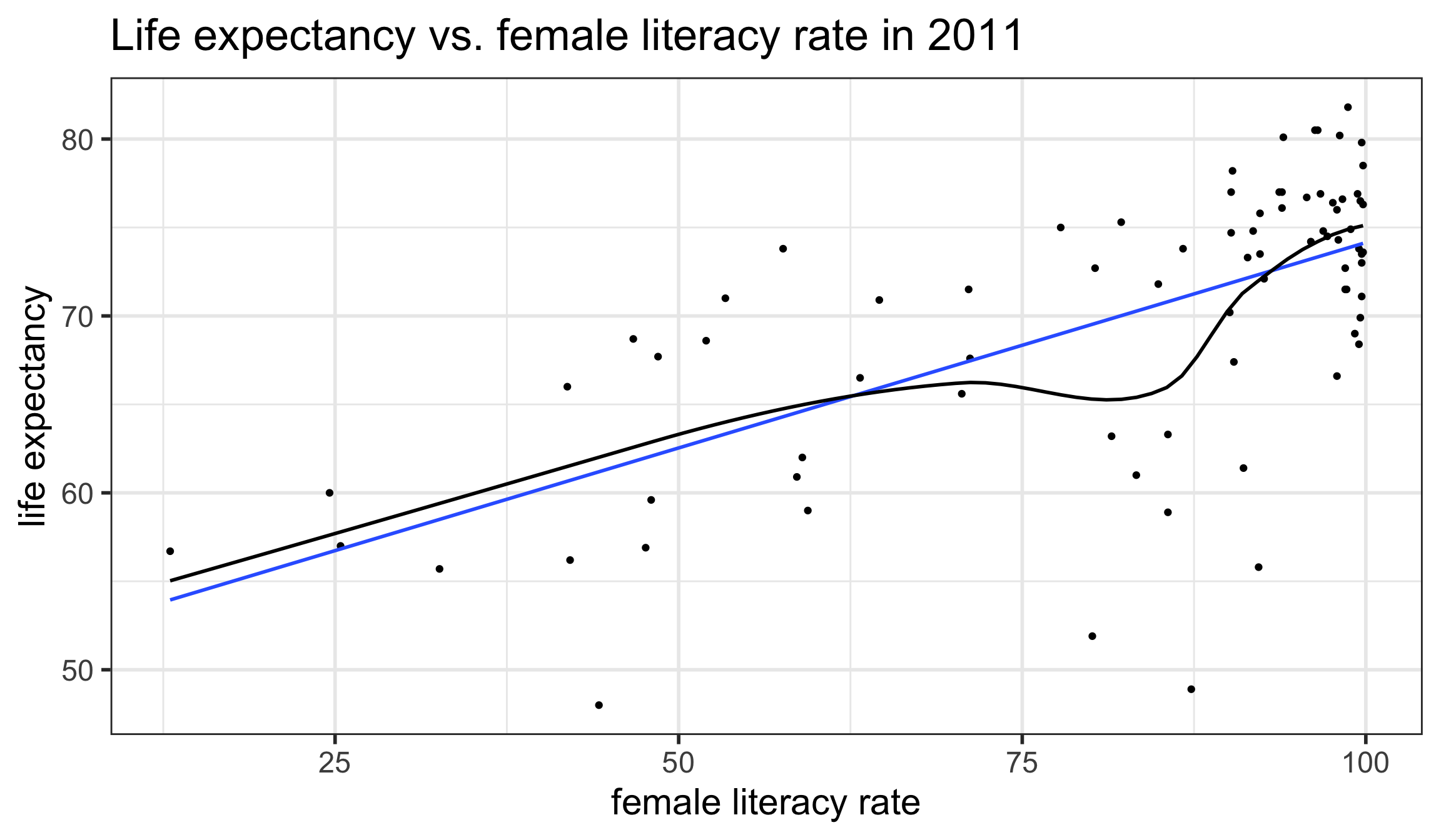
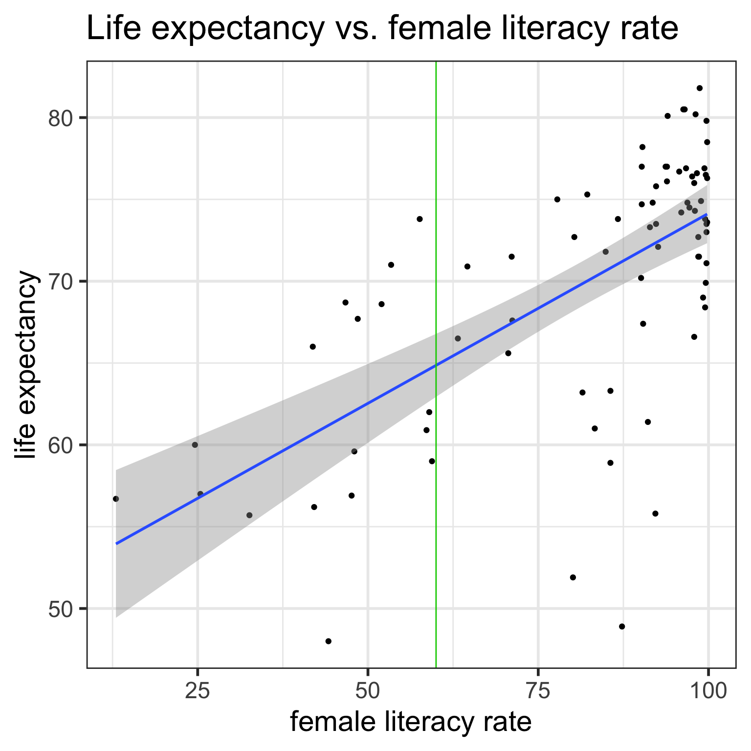
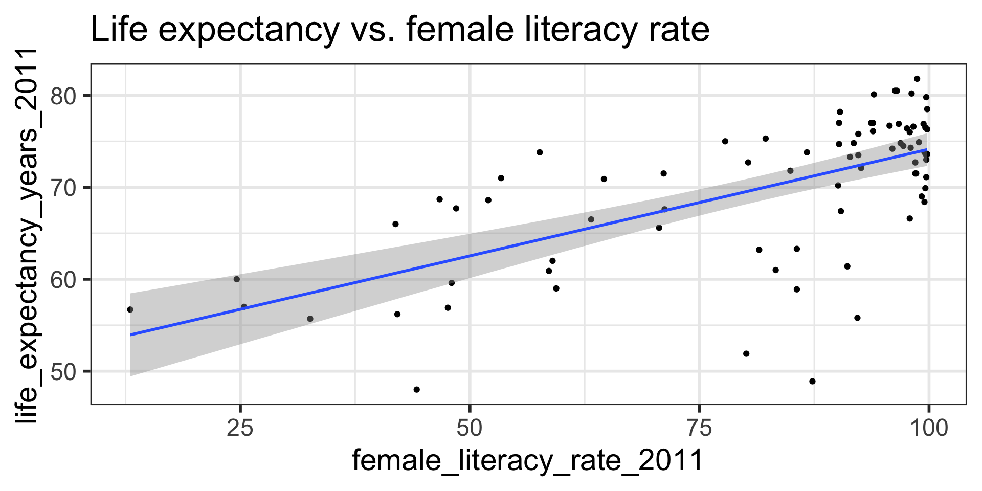
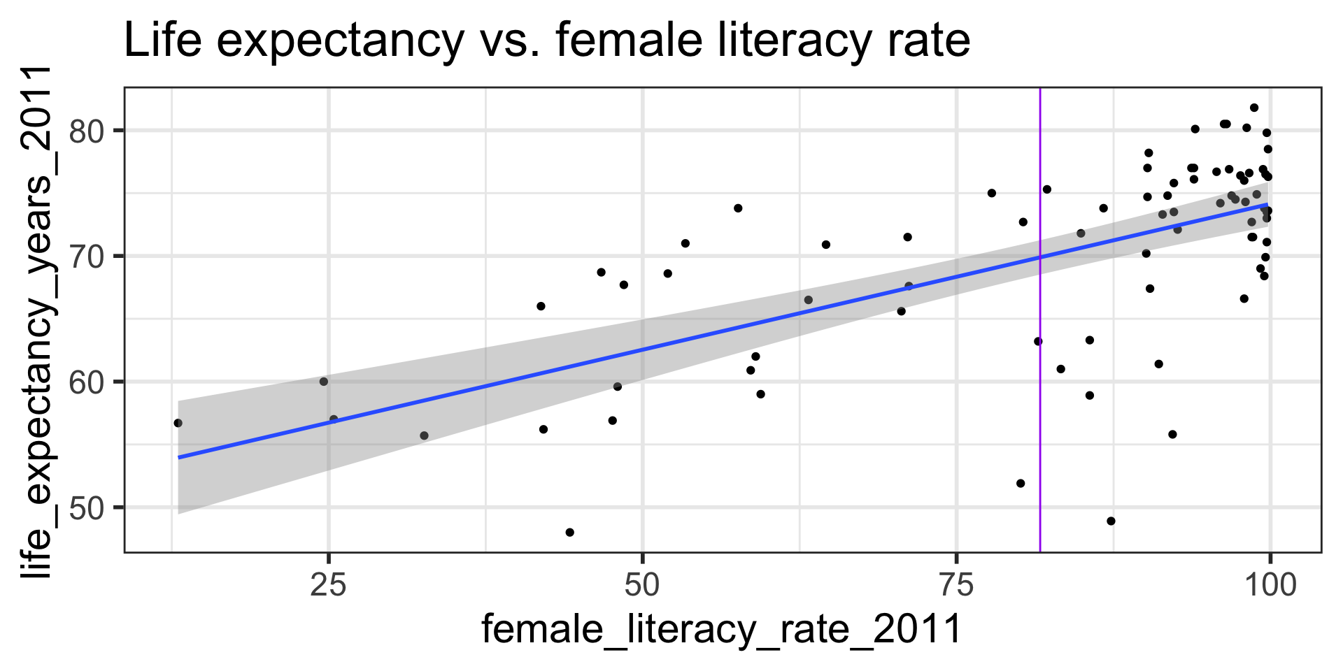
Life expectancy vs. female adult literacy rate
Regression line = best-fit line
\[\widehat{y} = b_0 + b_1 \cdot x \]
- \(\hat{y}\) is the predicted outcome for a specific value of \(x\).
- \(b_0\) is the intercept
- \(b_1\) is the slope of the line, i.e., the increase in \(\hat{y}\) for every increase of one (unit increase) in \(x\).
- slope = rise over run
- Intercept
- The expected outcome for the \(y\)-variable when the \(x\)-variable is 0.
- Slope
- For every increase of 1 unit in the \(x\)-variable, there is an expected increase of, on average, \(b_1\) units in the \(y\)-variable.
- We only say that there is an expected increase and not necessarily a causal increase.
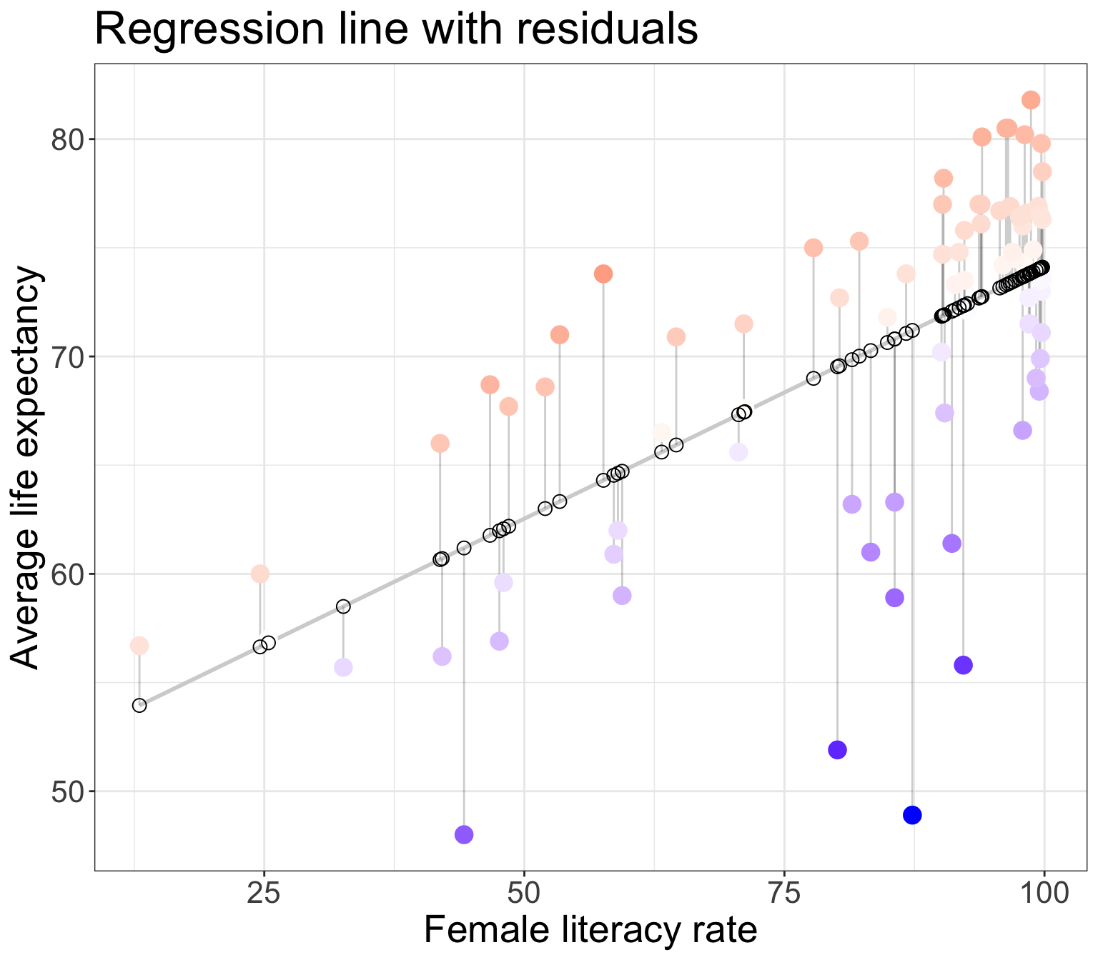
Residuals
- Observed values \(y_i\)
- the values in the dataset
- Fitted values \(\widehat{y}_i\)
- the values that fall on the best-fit line for a specific \(x_i\)
- Residuals \(e_i = y_i - \widehat{y}_i\)
- the differences between the observed and fitted values
The (population) regresison model
- The (population) regression model is denoted by
\[Y = \beta_0 + \beta_1 \cdot X + \epsilon\]
- \(\beta_0\) and \(\beta_1\) are unknown population parameters
- \(\epsilon\) (epsilon) is the error about the line
- It is assumed to be a random variable:
- \(\epsilon \sim N(0, \sigma^2)\)
- variance \(\sigma^2\) is constant
- It is assumed to be a random variable:
The line is the average (expected) value of \(Y\) given a value of \(x\): \(E(Y|x)\).
The point estimates for \(\beta_0\) and \(\beta_1\) based on a sample are denoted by \(b_0, b_1, s_{residuals}^2\)
- Note: also common notation is \(\widehat{\beta}_0, \widehat{\beta}_1, \widehat{\sigma}^2\)
L: Linearity of relationship between variables
Is the association between the variables linear?
- Diagnostic tools:
- Scatterplot
- Residual plot (see later section for E : Equality of variance of the residuals)
N: Normality of the residuals
- The responses Y are normally distributed at each level of x
Check normality with “usual” distribution plots
Note that below I save each figure, and then combine them together in one row of output using grid.arrange() from the gridExtra package.
Normal QQ plots (QQ = quantile-quantile)
- It can be tricky to eyeball with a histogram or density plot whether the residuals are normal or not
- QQ plots are often used to help with this
- Vertical axis: data quantiles
- data points are sorted in order and
- assigned quantiles based on how many data points there are
- Horizontal axis: theoretical quantiles
- mean and standard deviation (SD) calculated from the data points
- theoretical quantiles are calculated for each point, assuming the data are modeled by a normal distribution with the mean and SD of the data
- Data are approximately normal if points fall on a line.
See more info at https://data.library.virginia.edu/understanding-QQ-plots/
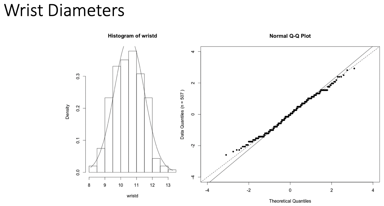
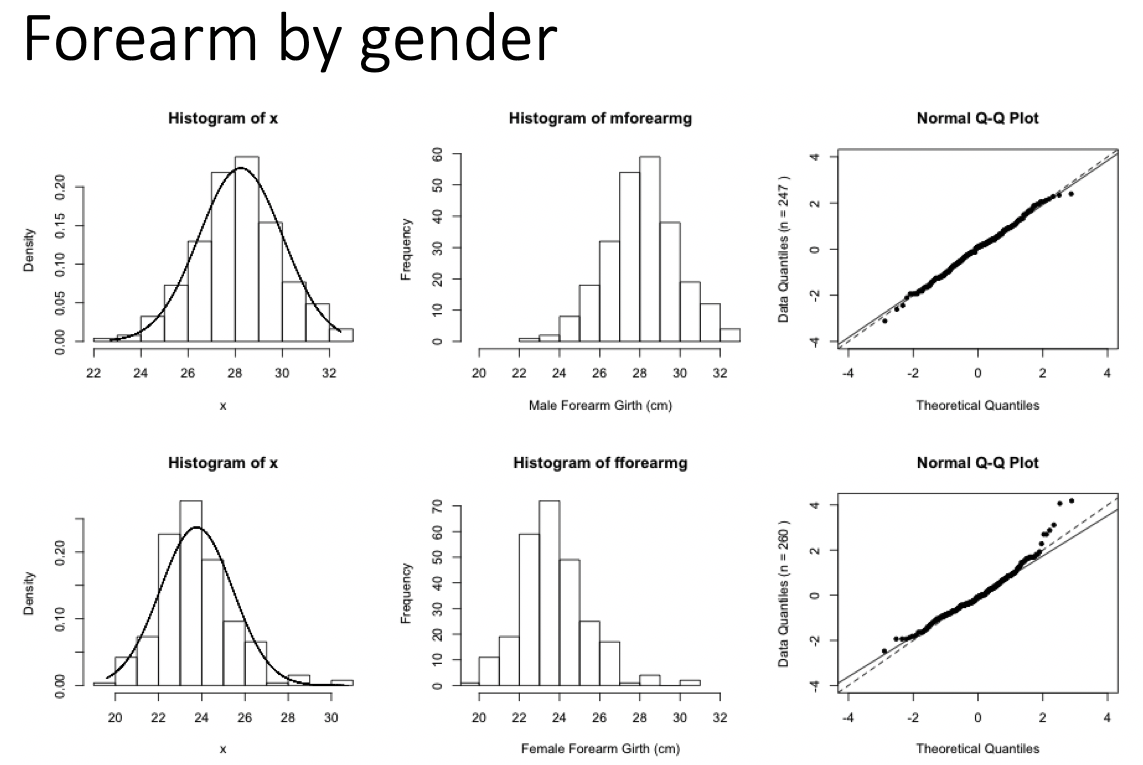
Examples of Normal QQ plots (1/5)
- Data:
- Body measurements from 507 physically active individuals
- in their 20’s or early 30’s
- within normal weight range.
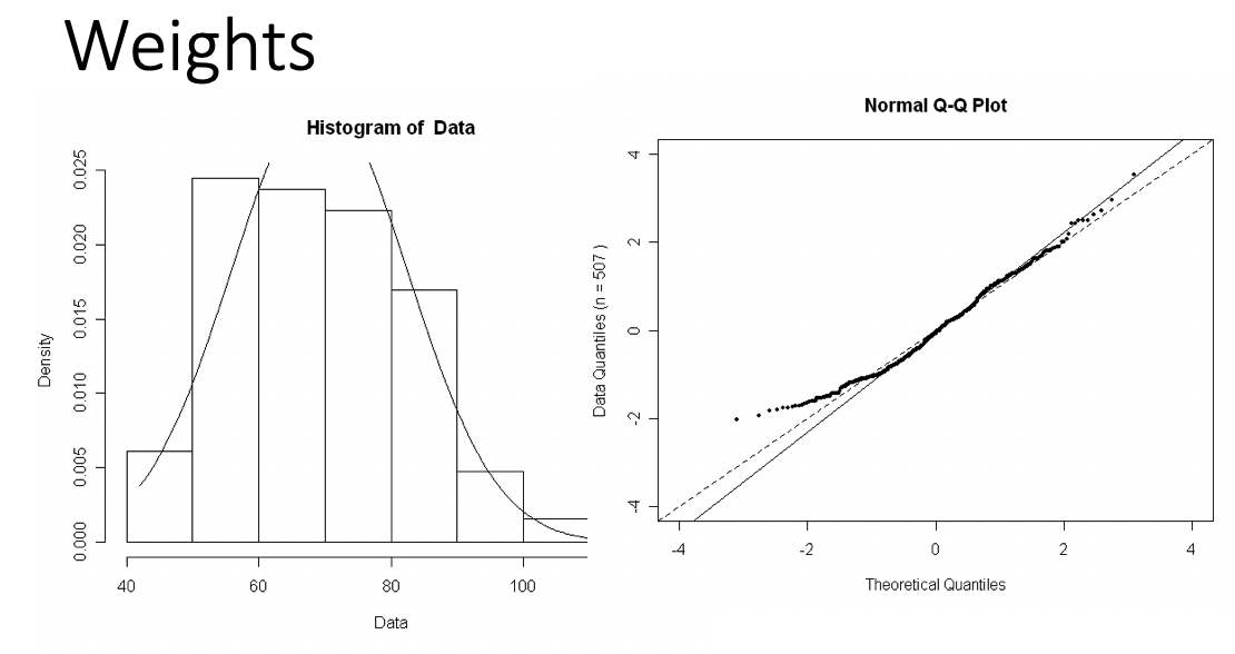
Examples of Normal QQ plots (2/5)
Skewed right distribution
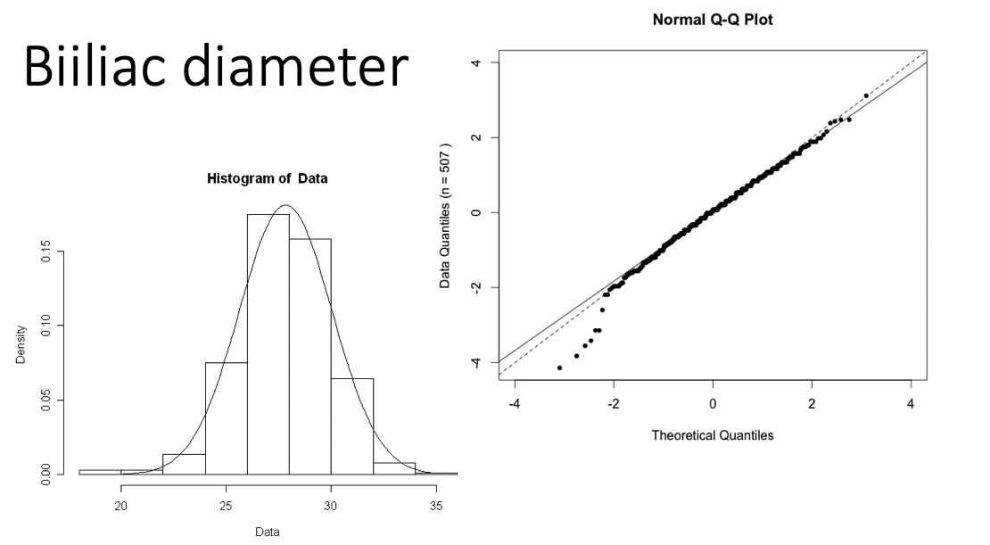
Examples of Normal QQ plots (3/5)
Long tails in distribution
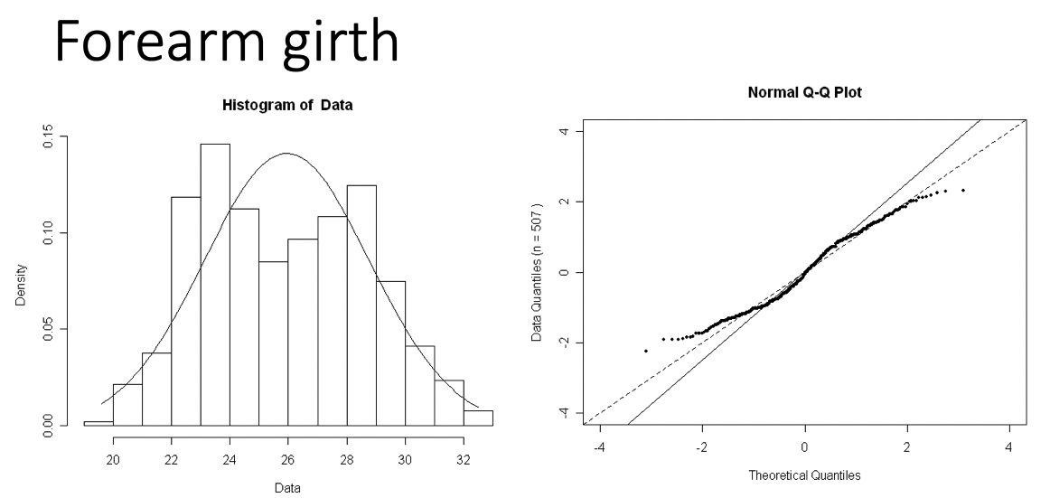
Examples of Normal QQ plots (4/5)
Bimodal distribution
Examples of Normal QQ plots (5/5)
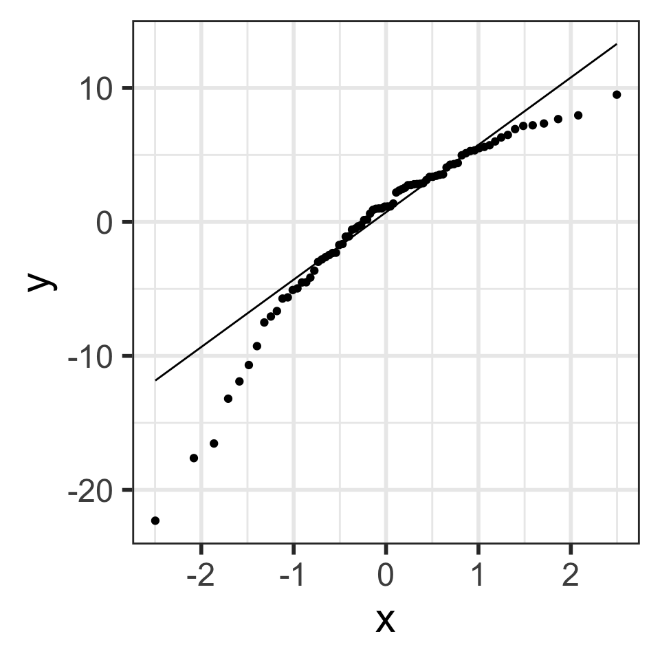
QQ plot of residuals of model1
Randomly generated Normal QQ plots: n=100
- Note that
stat_qq_line()doesn’t work with randomly generated samples, and thus the code below manually creates the line that the points should be on (which is \(y=x\) in this case.)
samplesize <- 100

rand_qq1 <- ggplot() +
  stat_qq(aes(sample = rnorm(samplesize))) +
  # line y=x
  geom_abline(intercept = 0, slope = 1,
              color = "blue")

rand_qq2 <- ggplot() +
  stat_qq(aes(sample = rnorm(samplesize))) +
  geom_abline(intercept = 0, slope = 1,
              color = "blue")

rand_qq3 <- ggplot() +
  stat_qq(aes(sample = rnorm(samplesize))) +
  geom_abline(intercept = 0, slope = 1,
              color = "blue")

rand_qq4 <- ggplot() +
  stat_qq(aes(sample = rnorm(samplesize))) +
  geom_abline(intercept = 0, slope = 1,
              color = "blue")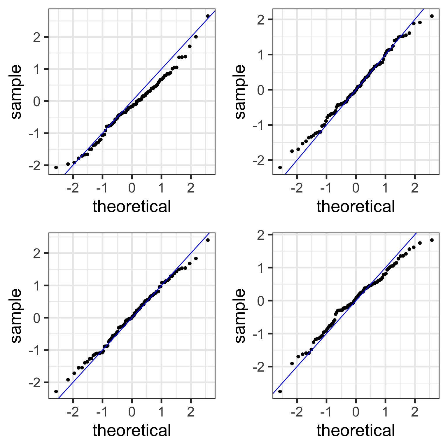
Examples of simulated Normal QQ plots: n=10
With fewer data points,
- simulated QQ plots are more likely to look “less normal”
- even though the data points were sampled from normal distributions.
samplesize <- 10  # only change made to code!

rand_qq1 <- ggplot() +
  stat_qq(aes(sample = rnorm(samplesize))) +
  # line y=x
  geom_abline(intercept = 0, slope = 1,
              color = "blue")

rand_qq2 <- ggplot() +
  stat_qq(aes(sample = rnorm(samplesize))) +
  geom_abline(intercept = 0, slope = 1,
              color = "blue")

rand_qq3 <- ggplot() +
  stat_qq(aes(sample = rnorm(samplesize))) +
  geom_abline(intercept = 0, slope = 1,
              color = "blue")

rand_qq4 <- ggplot() +
  stat_qq(aes(sample = rnorm(samplesize))) +
  geom_abline(intercept = 0, slope = 1,
              color = "blue")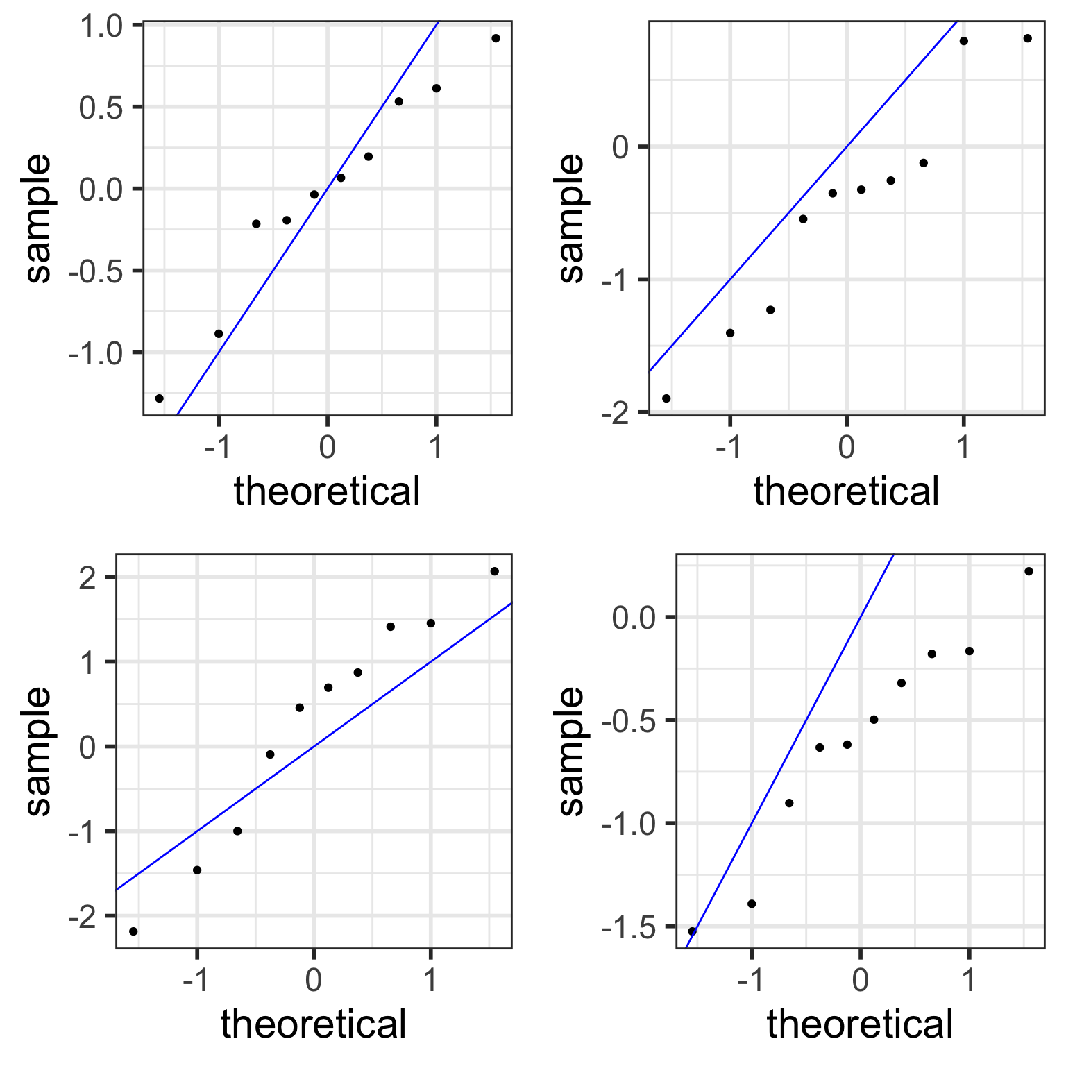
Examples of simulated Normal QQ plots: n=1,000
With more data points,
- simulated QQ plots are more likely to look “more normal”
samplesize <- 1000 # only change made to code!

rand_qq1 <- ggplot() +
  stat_qq(aes(sample = rnorm(samplesize))) +
  # line y=x
  geom_abline(intercept = 0, slope = 1,
              color = "blue")

rand_qq2 <- ggplot() +
  stat_qq(aes(sample = rnorm(samplesize))) +
  geom_abline(intercept = 0, slope = 1,
              color = "blue")

rand_qq3 <- ggplot() +
  stat_qq(aes(sample = rnorm(samplesize))) +
  geom_abline(intercept = 0, slope = 1,
              color = "blue")

rand_qq4 <- ggplot() +
  stat_qq(aes(sample = rnorm(samplesize))) +
  geom_abline(intercept = 0, slope = 1,
              color = "blue")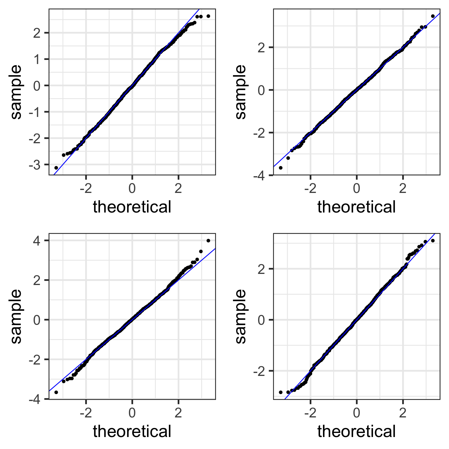
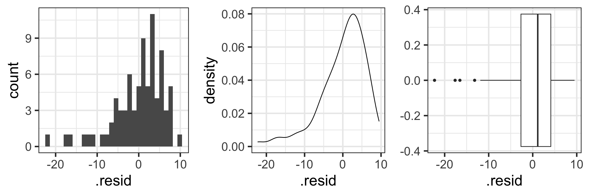
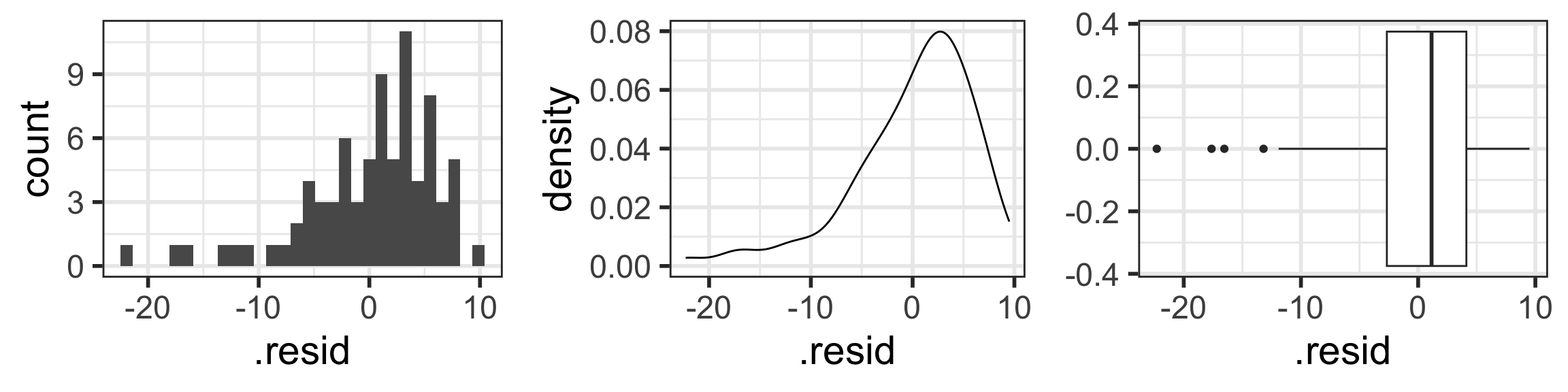
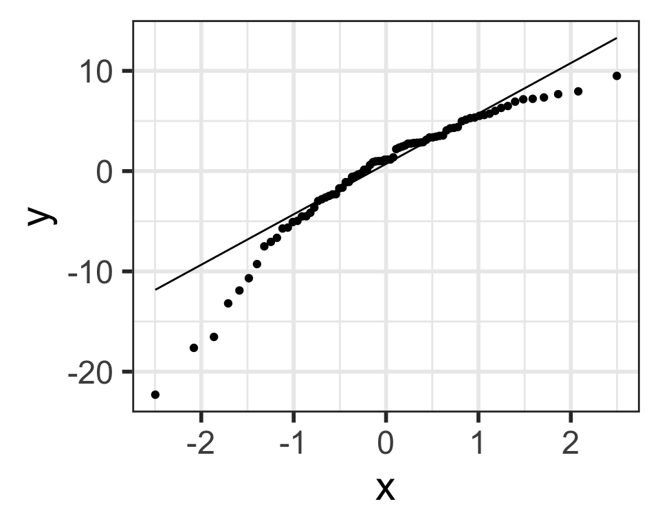
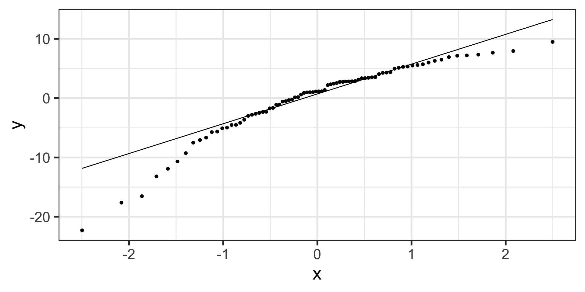
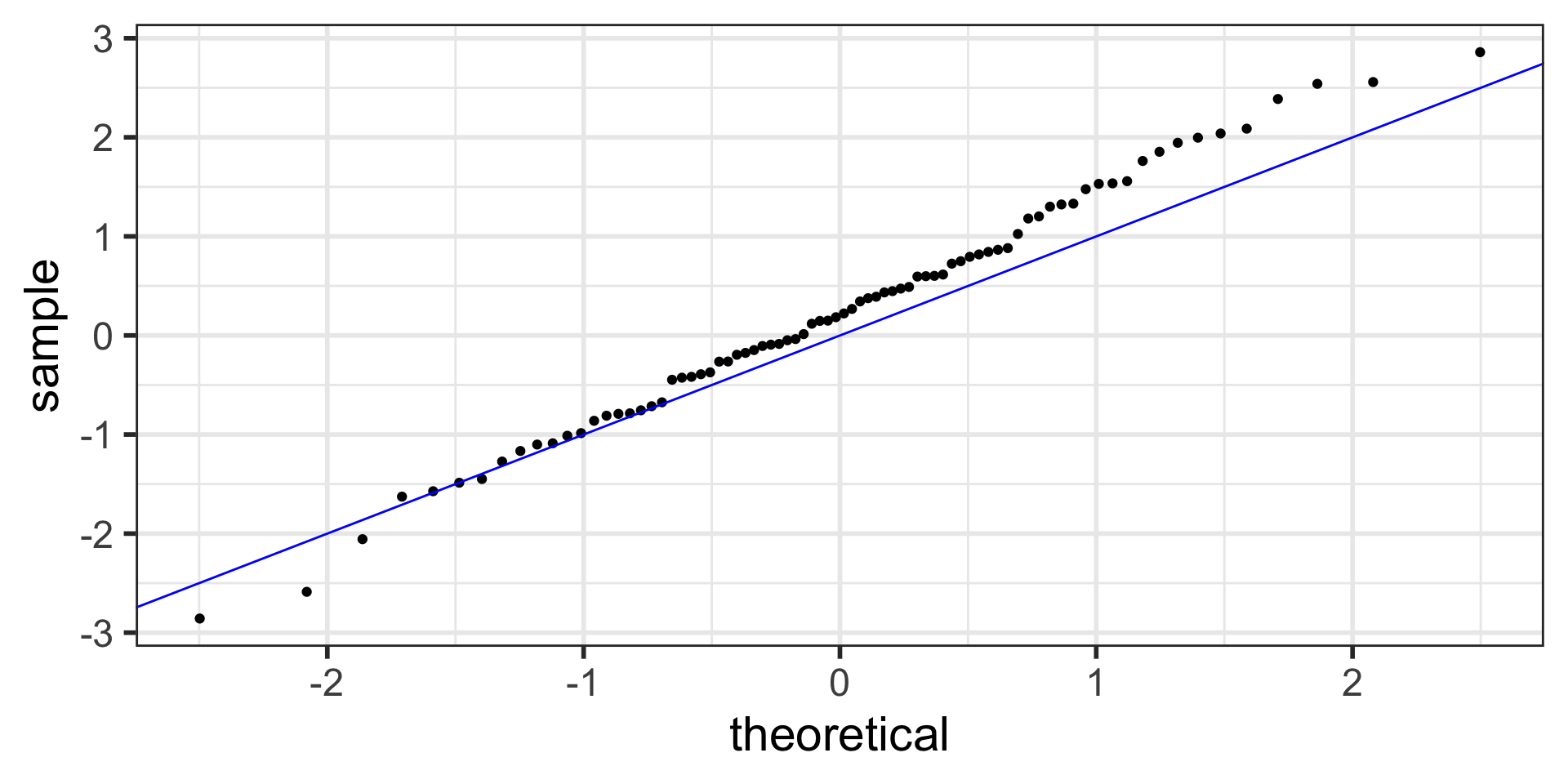
Back to our example
Residuals from Life Expectancy vs. Female Literacy Rate Regression
Simulated QQ plot of Normal Residuals with n = 80
E: Equality of variance of the residuals
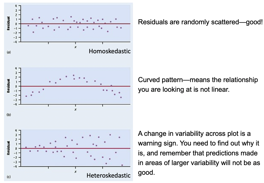
- Homoscedasticity
- Diagnostic tool: residual plot
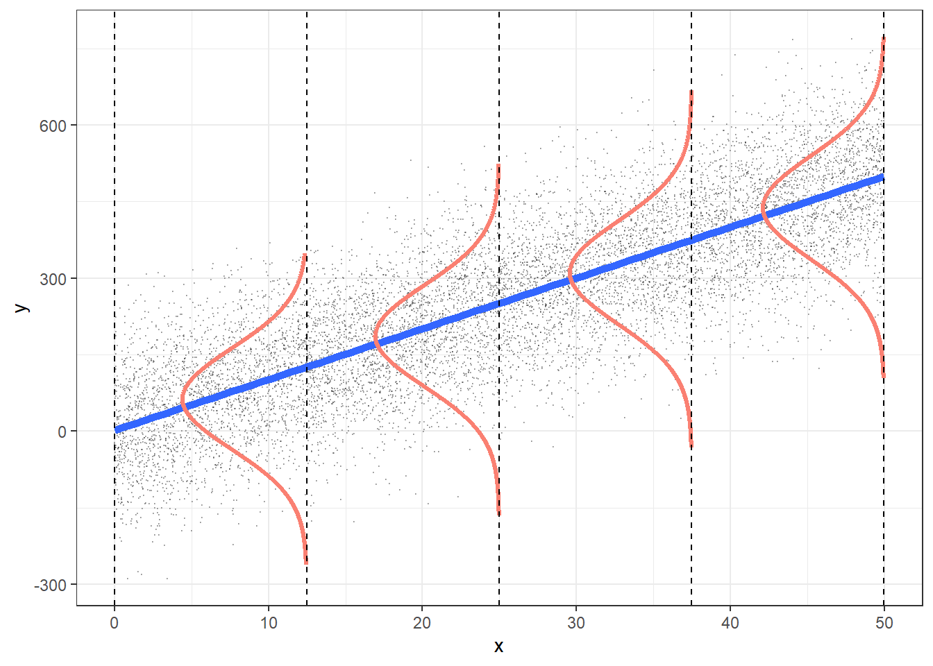
Residual plot
- \(x\) = explanatory variable from regression model
- (or the fitted values for a multiple regression)
- \(y\) = residuals from regression model
[1] "life_expectancy_years_2011" "female_literacy_rate_2011"
[3] ".fitted"                    ".resid"
[5] ".hat"                       ".sigma"
[7] ".cooksd" ".std.resid" 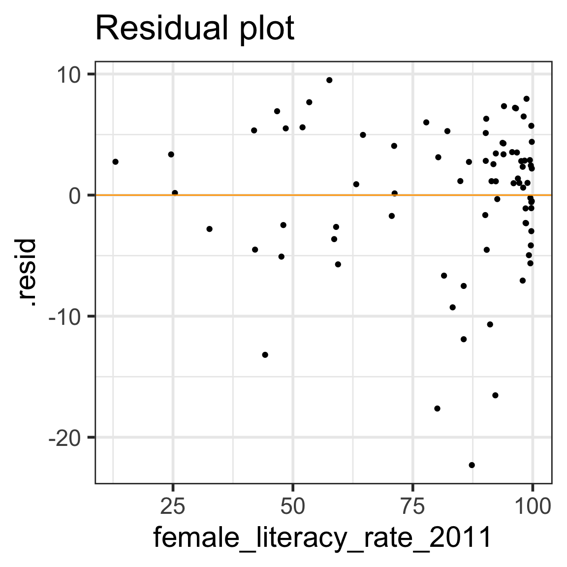
E: Equality of variance of the residuals (Homoscedasticity)
- The variance or, equivalently, the standard deviation of the responses is equal for all values of x.
- This is called homoskedasticity (top row)
- If there is heteroskedasticity (bottom row), then the assumption is not met.
Prediction with regression line
Recall the population model:
line + random “noise”
\[Y = \beta_0 + \beta_1 \cdot X + \varepsilon\] with \(\varepsilon \sim N(0,\sigma)\)
\(\sigma\) is the variability (SD) of the residuals
- When we take the expected value, at a given value \(x^*\), we have that the predicted response is the average expected response at \(x^*\):
\[\widehat{E[Y|x^*]} = b_0 + b_1 x^*\]
- These are the points on the regression line.
- The mean responses has variability, and we can calculate a CI for it, for every value of \(x^*\).
Confidence bands for mean response \(\mu_{Y|x^*}\)
- Often we plot the CI for many values of X, creating confidence bands
- The confidence bands are what ggplot creates when we set
se = TRUEwithingeom_smooth - For what values of x are the confidence bands (intervals) narrowest?
Width of confidence bands for mean response \(\mu_{Y|x^*}\)
- For what values of \(x^*\) are the confidence bands (intervals) narrowest? widest?
\[\begin{align} \widehat{E[Y|x^*]} &\pm t_{n-2}^* \cdot SE_{\widehat{E[Y|x^*]}}\\ \widehat{E[Y|x^*]} &\pm t_{n-2}^* \cdot s_{residuals} \sqrt{\frac{1}{n} + \frac{(x^* - \bar{x})^2}{(n-1)s_x^2}} \end{align}\]
Prediction bands vs. confidence bands (2/2)
 [1] "life_expectancy_years_2011" "female_literacy_rate_2011"
 [3] ".fitted"                    ".lower"
 [5] ".upper"                     ".resid"
 [7] ".hat"                       ".sigma"
[9] ".cooksd" ".std.resid" ggplot(model1_pred_bands,
aes(x=female_literacy_rate_2011, y=life_expectancy_years_2011)) +
geom_point() +
geom_ribbon(aes(ymin = .lower, ymax = .upper), # prediction bands
alpha = 0.2, fill = "red") +
geom_smooth(method=lm) + # confidence bands
labs(title = "SLR with Confidence & Prediction Bands") 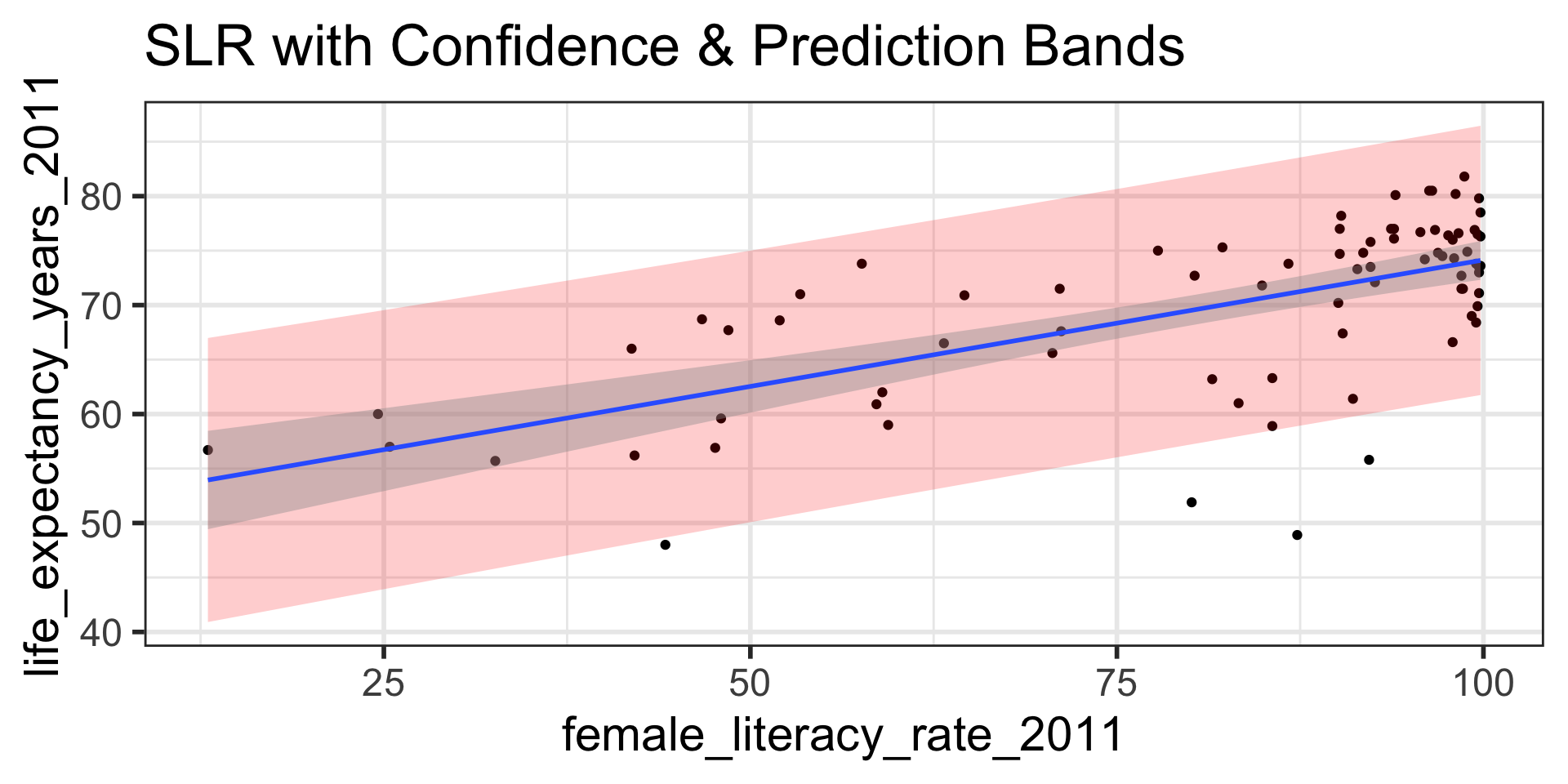
Corrrelation doesn’t imply causation*!
This might seem obvious, but make sure to not write your analysis results in a way that implies causation if the study design doesn’t warrant it (such as an observational study).
Beware of spurious correlations: http://www.tylervigen.com/spurious-correlations
*Caveat: there is a whole field of statistics/epidemiology on causal inference. https://ftp.cs.ucla.edu/pub/stat_ser/r350.pdf
What’s next?