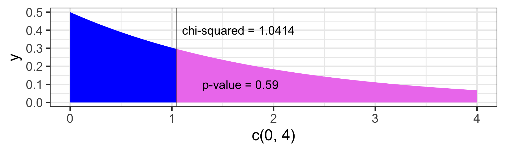
ggplot(NULL, aes(c(0,4))) +  # no dataset, create axes for x from 0 to 4
  geom_area(stat = "function", fun = dchisq, args = list(df=2),
            fill = "blue", xlim = c(0, 1.0414)) +
  geom_area(stat = "function", fun = dchisq, args = list(df=2),
            fill = "violet", xlim = c(1.0414, 4)) +
  geom_vline(xintercept = 1.0414) +  # vertical line at x = 1.0414
  annotate("text", x = 1.1, y = .4, # add text at specified (x,y) coordinate
           label = "chi-squared = 1.0414", hjust=0, size=6) +
  annotate("text", x = 1.3, y = .1,
label = "p-value = 0.59", hjust=0, size=6) Day 13: Chi-squared tests (Sections 8.3-8.4)
BSTA 511/611
2024-11-18
MoRitz’s tip of the day
Add text to a plot using annotate():
Where are we?
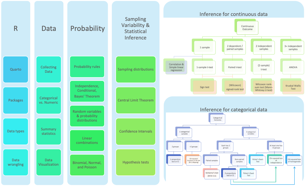
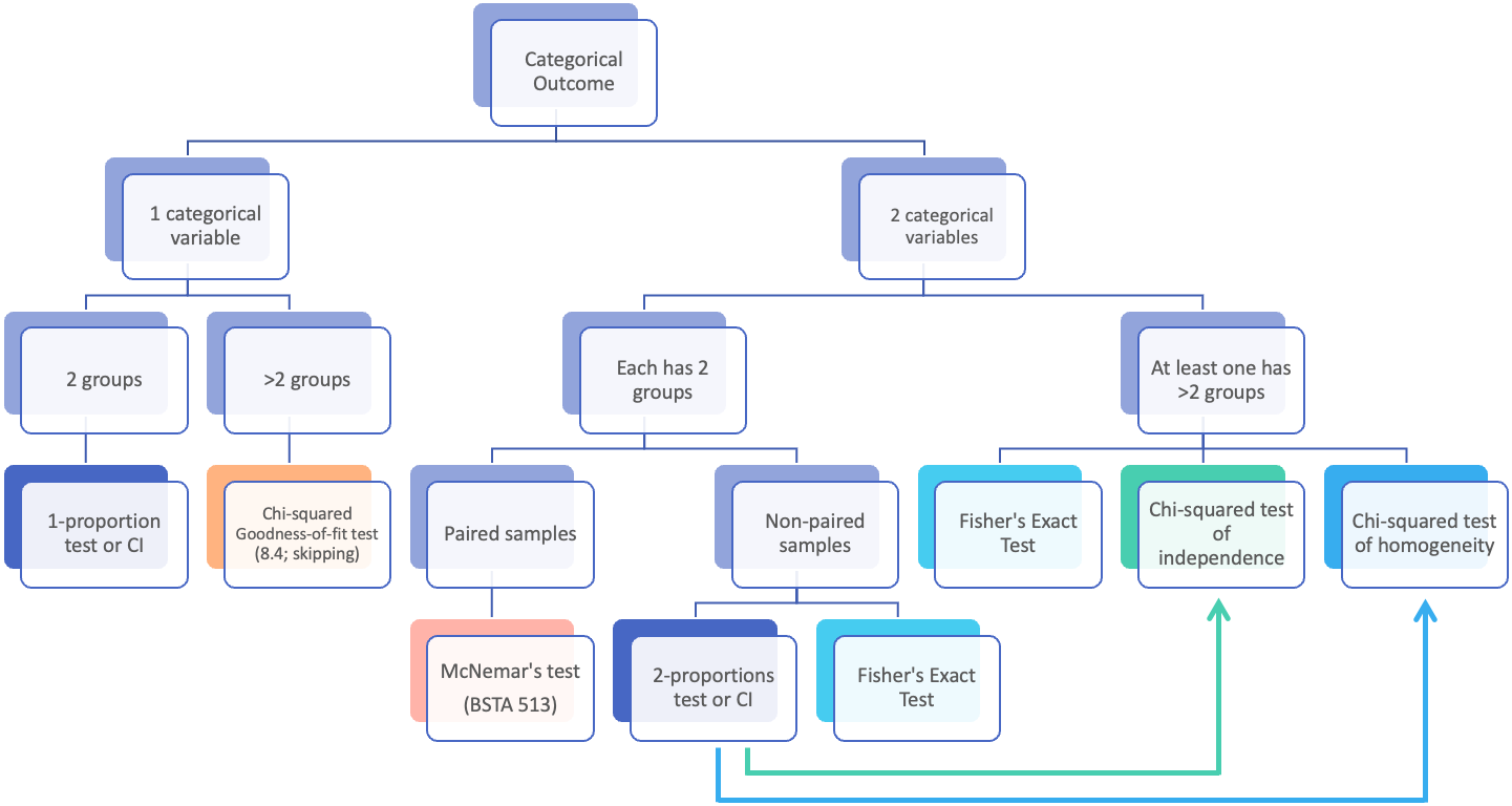
Where are we? Categorical outcome zoomed in
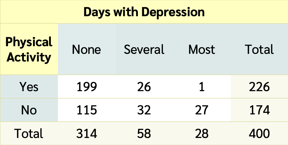
Data from NHANES
- Results below are from
- a random sample of 400 adults (≥ 18 yrs old)
- with data for both the depression
Depressedand physically active (PhysActive) variables.
- What does it mean for the variables to be independent?
\(H_0\): Variables are Independent
- Recall from Chapter 2, that events \(A\) and \(B\) are independent if and only if
\[P(A~and~B)=P(A)P(B)\]
- If depression and being physically active are independent variables, then theoretically this condition needs to hold for every combination of levels, i.e.
\[\begin{align} P(None~and~Yes) &= P(None)P(Yes)\\ P(None~and~No) &= P(None)P(No)\\ P(Several~and~Yes) &= P(Several)P(Yes)\\ P(Several~and~No) &= P(Several)P(No)\\ P(Most~and~Yes) &= P(Most)P(Yes)\\ P(Most~and~No) &= P(Most)P(No) \end{align}\]
\[\begin{align} P(None~and~Yes) &= \frac{314}{400}\cdot\frac{226}{400}\\ & ...\\ P(Most~and~No) &= \frac{28}{400}\cdot\frac{174}{400} \end{align}\]
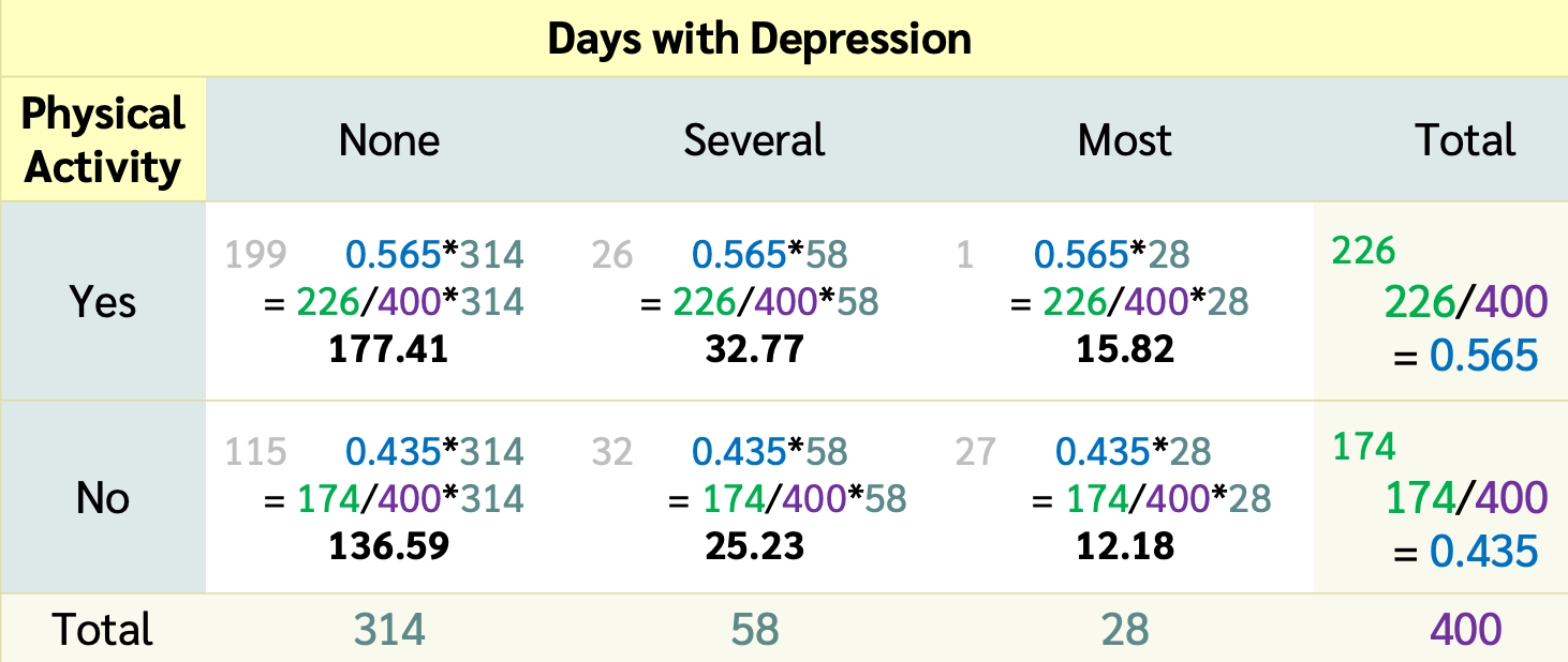
With these probabilities, for each cell of the table we calculate the expected counts for each cell under the \(H_0\) hypothesis that the variables are independent
Expected counts (if variables are independent)
- The expected counts (if \(H_0\) is true & the variables are independent) for each cell are
- \(np\) = total table size \(\cdot\) probability of cell
Expected count of Yes & None:
\[\begin{align} 400 \cdot & P(None~and~Yes)\\ &= 400 \cdot P(None)P(Yes)\\ &= 400 \cdot\frac{314}{400}\cdot\frac{226}{400}\\ &= \frac{314\cdot 226}{400} \\ &= 177.41\\ &= \frac{\text{column total}\cdot \text{row total}}{\text{table total}} \end{align}\]
- If depression and being physically active are independent variables
- (as assumed by \(H_0\)),
- then the observed counts should be close to the expected counts for each cell of the table
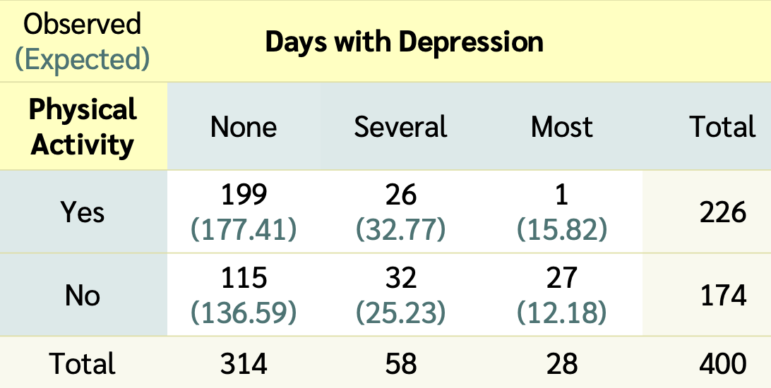
Observed vs. Expected counts
- The observed counts are the counts in the 2-way table summarizing the data
Expected count for cell \(i,j\) :
- The expected counts are the counts the we would expect to see in the 2-way table if there was no association between depression and being physically activity
\[\textrm{Expected Count}_{\textrm{row } i,\textrm{ col }j}=\frac{(\textrm{row}~i~ \textrm{total})\cdot(\textrm{column}~j~ \textrm{total})}{\textrm{table total}}\]
The \(\chi^2\) test statistic
Test statistic for a test of association (independence):
\[\chi^2 = \sum_{\textrm{all cells}} \frac{(\textrm{observed} - \text{expected})^2}{\text{expected}}\]
- When the variables are independent, the observed and expected counts should be close to each other
\[\begin{align} \chi^2 &= \sum\frac{(O-E)^2}{E} \\ &= \frac{(199-177.41)^2}{177.41} + \frac{(26-32.77)^2}{32.77} + \ldots + \frac{(27-12.18)^2}{12.18} \\ &= 41.2 \end{align}\]
Is this value big? Big enough to reject \(H_0\)?
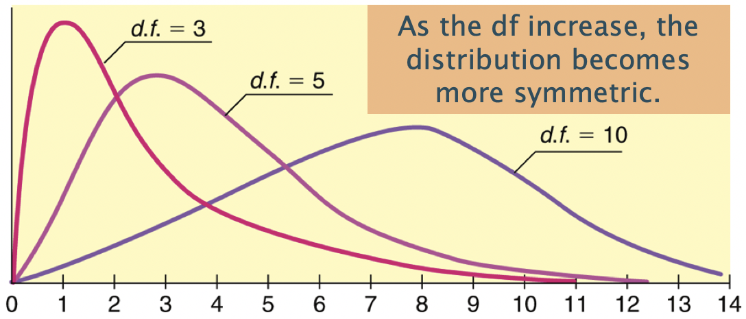
The \(\chi^2\) distribution & calculating the p-value
The \(\chi^2\) distribution shape depends on its degrees of freedom
- It’s skewed right for smaller df,
- gets more symmetric for larger df
- df = (# rows-1) x (# columns-1)
- The p-value is always the area to the right of the test statistic for a \(\chi^2\) test.
- We can use the
pchisqfunction in R to calculate the probability of being at least as big as the \(\chi^2\) test statistic:
What’s the conclusion to the \(\chi^2\) test?
Conclusion
Recall the hypotheses to our \(\chi^2\) test:
\(H_0\): There is no association between depression and being physically activity
\(H_A\): There is an association between depression and being physically activity
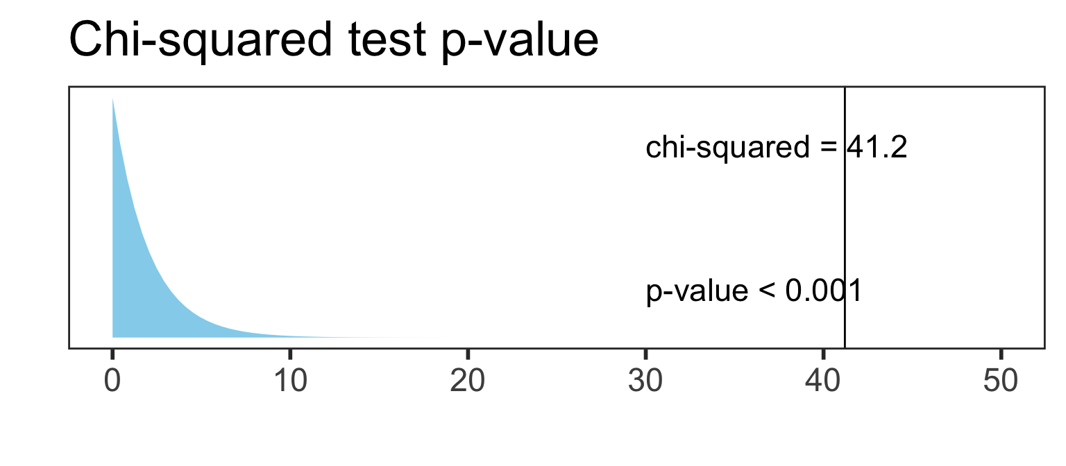
Conclusion:
Based a random sample of 400 US adults from 2009-2012, there is sufficient evidence that there is an association between depression and being physically activity (p-value < 0.001).
Warning
If we fail to reject, we DO NOT have evidence of no association.
Technical conditions
- Independence
- Each case (person) that contributes a count to the table must be independent of all the other cases in the table
- In particular, observational units cannot be represented in more than one cell.
- For example, someone cannot choose both “Several” and “Most” for depression status. They have to choose exactly one option for each variable.
- Each case (person) that contributes a count to the table must be independent of all the other cases in the table
- Sample size
- In order for the distribution of the test statistic to be appropriately modeled by a chi-squared distribution we need
- 2 \(\times\) 2 table:
- expected counts are at least 10 for each cell
- larger tables:
- no more than 1/5 of the expected counts are less than 5, and
- all expected counts are greater than 1
Depression vs. physical activity dataset
Create dataset based on results table:
Summary table of data:
Observed & expected counts in R
You can see what the observed and expected counts are from the saved chi-squared test results:
Why is it important to look at the expected counts?
What are we looking for in the expected counts?
Overview of tests with categorical outcome
Chi-squared Tests of Independence vs. Homogeneity vs. Goodness-of-fit
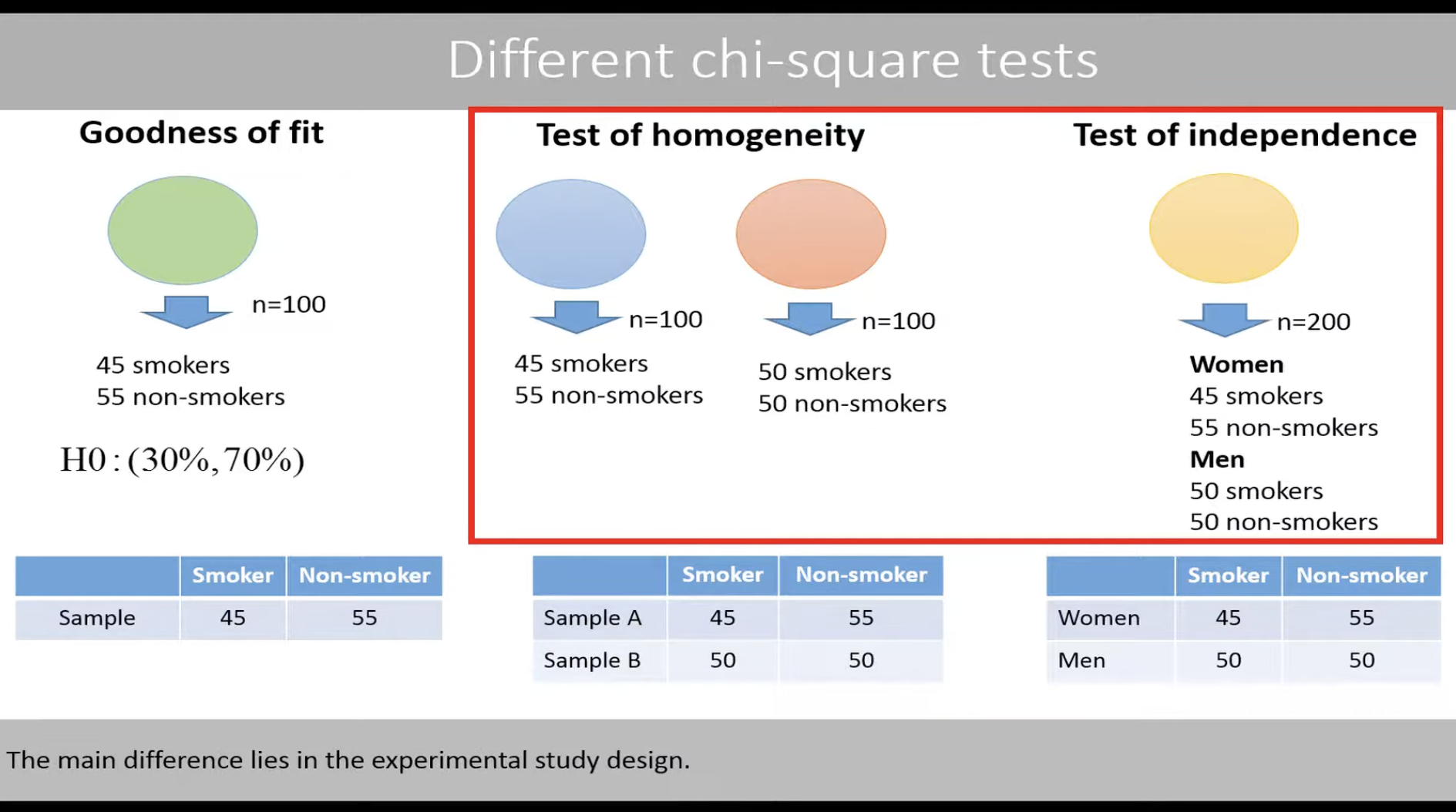
- See YouTube video from TileStats for a good explanation of how these three tests are different: https://www.youtube.com/watch?v=TyD-_1JUhxw
- UCLA’s INSPIRE website has a good summary too: http://inspire.stat.ucla.edu/unit_13/
What’s next?