Day 12: Inference for a single proportion or difference of two (independent) proportions (Sections 8.1-8.2)

BSTA 511/611

Meike Niederhausen, PhD

OHSU-PSU School of Public Health

2024-11-13

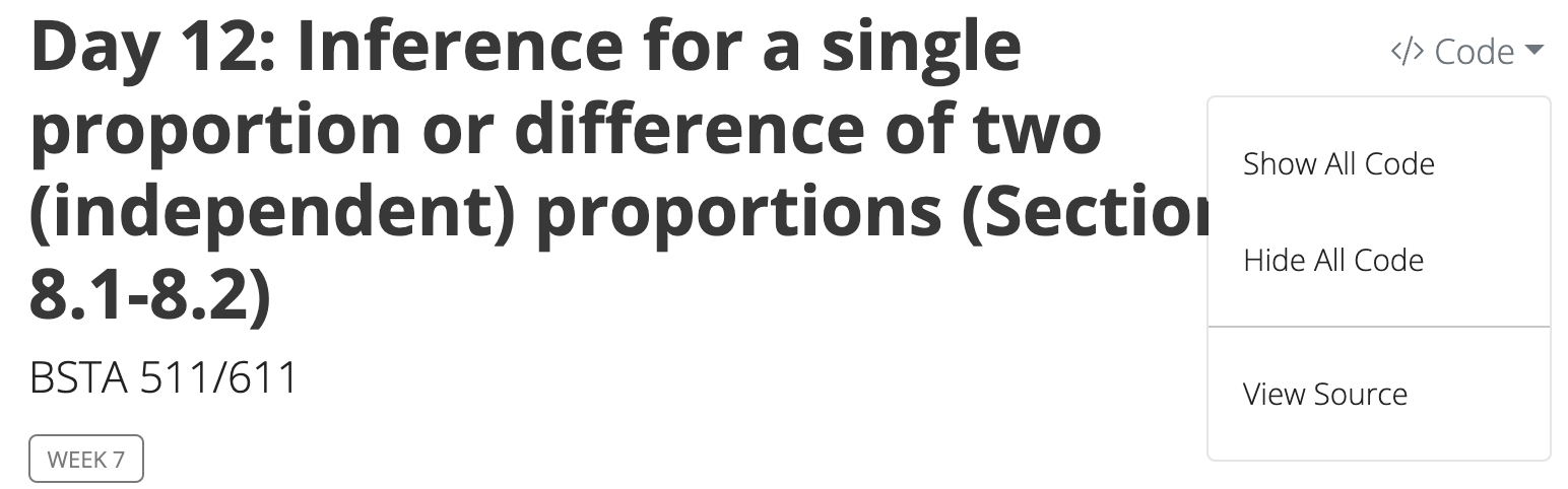
MoRitz’s tip of the day: code folding

• With code folding we can hide or show the code in the html output by clicking on the Code buttons in the html file.
• Note the </> Code button on the top right of the html output.

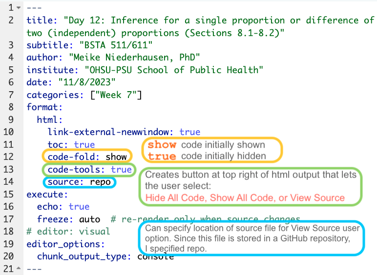
See more information at https://quarto.org/docs/output-formats/html-code.html#folding-code

Where are we?

CI’s and hypothesis tests for different scenarios:

\[\text{point estimate} \pm z^*(or~t^*)\cdot SE,~~\text{test stat} = \frac{\text{point estimate}-\text{null value}}{SE}\]

Day	Book	Population parameter	Symbol	Point estimate	Symbol	SE
10	5.1	Pop mean	\(\mu\)	Sample mean	\(\bar{x}\)	\(\frac{s}{\sqrt{n}}\)
10	5.2	Pop mean of paired diff	\(\mu_d\) or \(\delta\)	Sample mean of paired diff	\(\bar{x}_{d}\)	\(\frac{s_d}{\sqrt{n}}\)
11	5.3	Diff in pop means	\(\mu_1-\mu_2\)	Diff in sample means	\(\bar{x}_1 - \bar{x}_2\)	\(\sqrt{\frac{s_1^2}{n_1} + \frac{s_2^2}{n_2}}\) or pooled
12	8.1	Pop proportion	\(p\)	Sample prop	\(\widehat{p}\)	???
12	8.2	Diff in pop proportions	\(p_1-p_2\)	Diff in sample proportions	\(\widehat{p}_1-\widehat{p}_2\)	???

Goals for today (Sections 8.1-8.2)

• Statistical inference for a single proportion or the difference of two (independent) proportions

  1. Sampling distribution for a proportion or difference in proportions

  2. What are \(H_0\) and \(H_a\)?

  3. What are the SE’s for \(\hat{p}\) and \(\hat{p}_1-\hat{p}_2\)?

  4. Hypothesis test

  5. Confidence Interval

  6. How are the SE’s different for a hypothesis test & CI?

  7. How to run proportions tests in R

  8. Power & sample size for proportions tests (extra material)

Motivating example

One proportion

• A 2010 study found that out of 269 male college students, 35% had participated in sports betting in the previous year.
  • What is the CI for the proportion?
  • The study also reported that 36% of noncollege young males had participated in sports betting. Is the proportion for male college students different from 0.36?

Two proportions

• There were 214 men in the sample of noncollege young males (36% participated in sports betting in the previous year).
• Compare the difference in proportions between the college and noncollege young males.
  • CI & Hypothesis test

Barnes GM, Welte JW, Hoffman JH, Tidwell MC. Comparisons of gambling and alcohol use among college students and noncollege young people in the United States. J Am Coll Health. 2010 Mar-Apr;58(5):443-52. doi: 10.1080/07448480903540499. PMID: 20304756; PMCID: PMC4104810.

Steps in a Hypothesis Test

1. Set the level of significance \(\alpha\)

2. Specify the null ( \(H_0\) ) and alternative ( \(H_A\) ) hypotheses

   1. In symbols
   2. In words
   3. Alternative: one- or two-sided?

3. Calculate the test statistic.

4. Calculate the p-value based on the observed test statistic and its sampling distribution

5. Write a conclusion to the hypothesis test

   1. Do we reject or fail to reject \(H_0\)?
   2. Write a conclusion in the context of the problem

Step 2: Null & Alternative Hypotheses

Null and alternative hypotheses in words and in symbols.

One sample test

• \(H_0\): The population proportion of young male college students that participated in sports betting in the previous year is 0.36.

• \(H_A\): The population proportion of young male college students that participated in sports betting in the previous year is not 0.36.

\[\begin{align} H_0:& p = 0.36\\ H_A:& p \neq 0.36\\ \end{align}\]

Two samples test

• \(H_0\): The difference in population proportions of young male college and noncollege students that participated in sports betting in the previous year is 0.

• \(H_A\): The difference in population proportions of young male college and noncollege students that participated in sports betting in the previous year is not 0.

\[\begin{align} H_0:& p_{coll} - p_{noncoll} = 0\\ H_A:& p_{coll} - p_{noncoll} \neq 0\\ \end{align}\]

Sampling distribution of \(\hat{p}\)

• \(\hat{p}=\frac{X}{n}\) where \(X\) is the number of “successes” and \(n\) is the sample size.
• \(X \sim Bin(n,p)\), where \(p\) is the population proportion.
• For \(n\) “big enough”, the normal distribution can be used to approximate a binomial distribution:

\[Bin(n,p) \rightarrow N\Big(\mu = np, \sigma = \sqrt{np(1-p)} \Big)\]

• Since \(\hat{p}=\frac{X}{n}\) is a linear transformation of \(X\), we have for large n:

\[\hat{p} \sim N\Big(\mu_{\hat{p}} = p, \sigma_{\hat{p}} = \sqrt{\frac{p(1-p)}{n}} \Big)\]

• How we apply this result to CI’s and test statistics is different!!!

Step 3: Test statistic

Sampling distribution of \(\hat{p}\) if we assume \(H_0: p=p_0\) is true:

\[\hat{p} \sim N\Big(\mu_{\hat{p}} = p, \sigma_{\hat{p}} = \sqrt{\frac{p(1-p)}{n}} \Big) \sim N\Big( \mu_{\hat{p}}=p_0, \sigma_{\hat{p}}=\sqrt{\frac{p_0\cdot(1-p_0)}{n}} \Big)\]

Test statistic for a one sample proportion test:

\[ \text{test stat} = \frac{\text{point estimate}-\text{null value}}{SE} = z_{\hat{p}} = \frac{\hat{p} - p_0}{\sqrt{\frac{p_0\cdot(1-p_0)}{n}}} \]

---

Example: A 2010 study found that out of 269 male college students, 35% had participated in sports betting in the previous year.

What is the test statistic when testing \(H_0: p=0.36\) vs.  \(H_A: p \neq 0.36\)?

\[\begin{align} z_{\hat{p}} &= \frac{94/269 - 0.36}{\sqrt{\frac{0.36\cdot(1-0.36)}{269}}} \\ & -0.3607455 \end{align}\]

Step “3b”: Conditions satisfied?

Conditions:

1. Independent observations?
   • The observations were collected independently.
2. The number of expected successes and expected failures is at least 10.
   • \(n_1 p_0 \ge 10, \ \ n_1(1-p_0)\ge 10\)

---

Example: A 2010 study found that out of 269 male college students, 35% had participated in sports betting in the previous year.

Testing \(H_0: p=0.36\) vs. \(H_A: p \neq 0.36\).

Are the conditions satisfied?

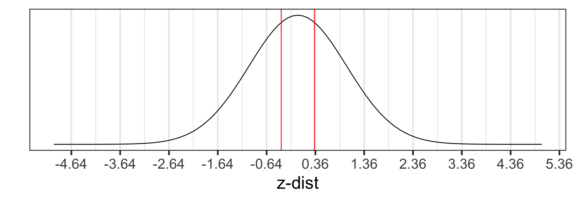
Step 4: p-value

The p-value is the probability of obtaining a test statistic just as extreme or more extreme than the observed test statistic assuming the null hypothesis \(H_0\) is true.

Calculate the p-value:

\[\begin{align} 2 &\cdot P(\hat{p}<0.35) \\ &= 2 \cdot P\Big(Z_{\hat{p}} < \frac{94/269 - 0.36}{\sqrt{\frac{0.36\cdot(1-0.36)}{269}}}\Big)\\ &=2 \cdot P(Z_{\hat{p}} < -0.3607455)\\ &= 0.7182897 \end{align}\]

2*pnorm(-0.3607455)

[1] 0.7182897

Step 5: Conclusion to hypothesis test

\[\begin{align} H_0:& p = 0.36\\ H_A:& p \neq 0.36\\ \end{align}\]

• Recall the \(p\)-value = 0.7182897
• Use \(\alpha\) = 0.05.
• Do we reject or fail to reject \(H_0\)?

Conclusion statement:

• Stats class conclusion
  • There is insufficient evidence that the (population) proportion of young male college students that participated in sports betting in the previous year is different than 0.36 ( \(p\)-value = 0.72).
• More realistic manuscript conclusion:
  • In a sample of 269 male college students, 35% had participated in sports betting in the previous year, which is not different from 36% ( \(p\)-value = 0.72).

95% CI for population proportion

What to use for SE in CI formula?

\[\hat{p} \pm z^* \cdot SE_{\hat{p}}\]

Sampling distribution of \(\hat{p}\):

\[\hat{p} \sim N\Big(\mu_{\hat{p}} = p, \sigma_{\hat{p}} = \sqrt{\frac{p(1-p)}{n}} \Big)\]

Problem: We don’t know what \(p\) is - it’s what we’re estimating with the CI.
Solution: approximate \(p\) with \(\hat{p}\):

\[SE_{\hat{p}} = \sqrt{\frac{\hat{p}(1-\hat{p})}{n}}\]

---

Example: A 2010 study found that out of 269 male college students, 35% had participated in sports betting in the previous year.
Find the 95% CI for the population proportion.

\[\begin{align} 94/269 &\pm 1.96 \cdot SE_{\hat{p}}\\ SE_{\hat{p}} &= \sqrt{\frac{(94/269)(1-94/269)}{269}}\\ (0.293 &, 0.407) \end{align}\]

Interpretation:
We are 95% confident that the (population) proportion of young male college students that participated in sports betting in the previous year is in (0.29, 0.41).

Conditions for one proportion: test vs. CI

Hypothesis test conditions

1. Independent observations
   • The observations were collected independently.

2. The number of expected successes and expected failures is at least 10.

\[n_1 p_0 \ge 10, \ \ n_1(1-p_0)\ge 10\]

Confidence interval conditions

1. Independent observations
   • The observations were collected independently.

2. The number of successes and failures is at least 10:

\[n_1\hat{p}_1 \ge 10, \ \ n_1(1-\hat{p}_1)\ge 10\]

Inference for difference of two independent proportions
\(\hat{p}_1-\hat{p}_2\)

Sampling distribution of \(\hat{p}_1-\hat{p}_2\)

• \(\hat{p}_1=\frac{X_1}{n_1}\) and \(\hat{p}_2=\frac{X_2}{n_2}\),
  • \(X_1\) & \(X_2\) are the number of “successes”
  • \(n_1\) & \(n_2\) are the sample sizes of the 1st & 2nd samples

• Each \(\hat{p}\) can be approximated by a normal distribution, for “big enough” \(n\)
• Since the difference of independent normal random variables is also normal, it follows that for “big enough” \(n_1\) and \(n_2\)

\[\hat{p}_1 - \hat{p}_2 \sim N \Big(\mu_{\hat{p}_1 - \hat{p}_2} = p_1 - p_2, ~~ \sigma_{\hat{p}_1 - \hat{p}_2} = \sqrt{ \frac{p_1\cdot(1-p_1)}{n_1} + \frac{p_2\cdot(1-p_2)}{n_2}} \Big)\]

where \(p_1\) & \(p_2\) are the population proportions, respectively.

• How we apply this result to CI’s and test statistics is different!!!

Step 3: Test statistic (1/2)

Sampling distribution of \(\hat{p}_1 - \hat{p}_2\): \[\hat{p}_1 - \hat{p}_2 \sim N \Big(\mu_{\hat{p}_1 - \hat{p}_2} = p_1 - p_2, ~~ \sigma_{\hat{p}_1 - \hat{p}_2} = \sqrt{ \frac{p_1\cdot(1-p_1)}{n_1} + \frac{p_2\cdot(1-p_2)}{n_2}} \Big)\]

Since we assume \(H_0: p_1 - p_2 = 0\) is true, we “pool” the proportions of the two samples to calculate the SE:

\[\text{pooled proportion} = \hat{p}_{pool} = \dfrac{\text{total number of successes} }{ \text{total number of cases}} = \frac{x_1+x_2}{n_1+n_2}\]

Test statistic:

\[ \text{test statistic} = z_{\hat{p}_1 - \hat{p}_2} = \frac{\hat{p}_1 - \hat{p}_2 - 0}{\sqrt{\frac{\hat{p}_{pool}\cdot(1-\hat{p}_{pool})}{n_1} + \frac{\hat{p}_{pool}\cdot(1-\hat{p}_{pool})}{n_2}}} \]

Step 3: Test statistic (2/2)

\[ \text{test statistic} = z_{\hat{p}_1 - \hat{p}_2} = \frac{\hat{p}_1 - \hat{p}_2 - 0}{\sqrt{\frac{\hat{p}_{pool}\cdot(1-\hat{p}_{pool})}{n_1} + \frac{\hat{p}_{pool}\cdot(1-\hat{p}_{pool})}{n_2}}} \]

\[\text{pooled proportion} = \hat{p}_{pool} = \dfrac{\text{total number of successes} }{ \text{total number of cases}} = \frac{x_1+x_2}{n_1+n_2}\]

---

Example: A 2010 study found that out of 269 male college students, 35% had participated in sports betting in the previous year, and out of 214 noncollege young males 36% had.
What is the test statistic when testing \(H_0: p_{coll} - p_{noncoll} = 0\) vs.  \(H_A: p_{coll} - p_{noncoll} \neq 0\)?

\[\begin{align} z_{\hat{p}_1 - \hat{p}_2} &= \frac{94/269 - 77/214-0}{\sqrt{0.354\cdot(1-0.354)(\frac{1}{269}+\frac{1}{214})}}\\ &=-0.2367497 \end{align}\]

Step “3b”: Conditions satisfied?

Conditions:

• Independent observations & samples
  • The observations were collected independently.
  • In particular, observations from the two groups weren’t paired in any meaningful way.
• The number of expected successes and expected failures is at least 10 for each group - using the pooled proportion:
  • \(n_1\hat{p}_{pool} \ge 10, \ \ n_1(1-\hat{p}_{pool}) \ge 10\)
  • \(n_2\hat{p}_{pool} \ge 10, \ \ n_2(1-\hat{p}_{pool}) \ge 10\)

Example: A 2010 study found that out of 269 male college students, 35% had participated in sports betting in the previous year, and out of 214 noncollege young males 36% had.
Testing \(H_0: p_{coll} - p_{noncoll} = 0\) vs.  \(H_A: p_{coll} - p_{noncoll} \neq 0\)? .

Are the conditions satisfied?

Step 4: p-value

The p-value is the probability of obtaining a test statistic just as extreme or more extreme than the observed test statistic assuming the null hypothesis \(H_0\) is true.

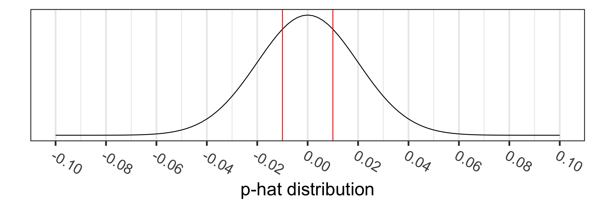
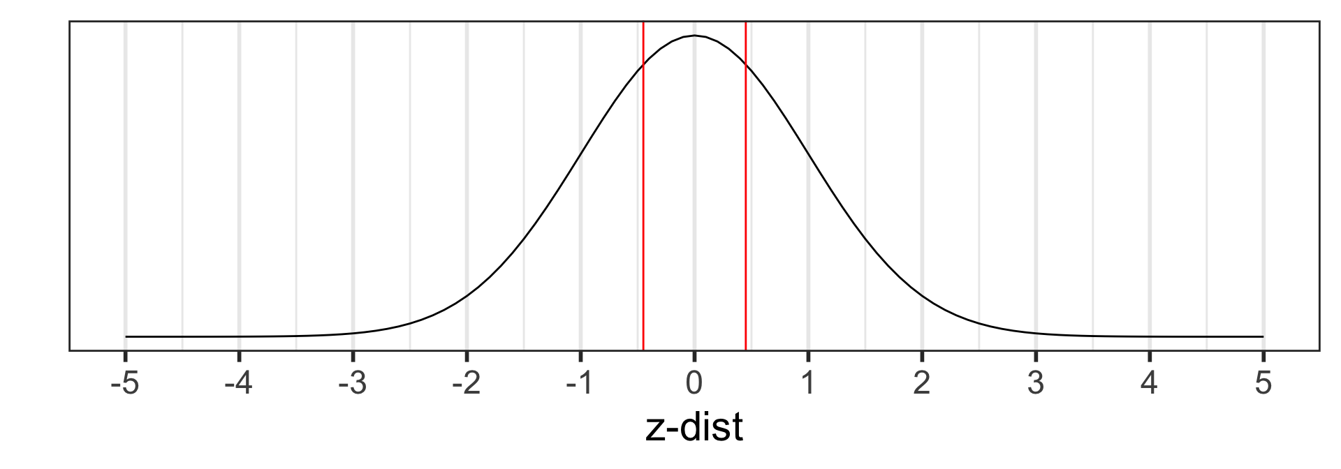
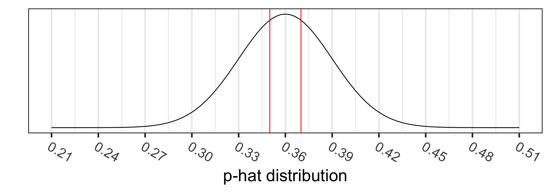
Calculate the p-value:

\[\begin{align} 2 &\cdot P(\hat{p}_1 - \hat{p}_2<0.35-0.36) \\ = 2 &\cdot P\Big(Z_{\hat{p}_1 - \hat{p}_2} < \\ &\frac{94/269 - 77/214-0}{\sqrt{0.354\cdot(1-0.354)(\frac{1}{269}+\frac{1}{214})}}\Big)\\ =2 &\cdot P(Z_{\hat{p}} < -0.2367497) \\ = & 0.812851 \end{align}\]

2*pnorm(-0.2367497)

[1] 0.812851

Step 5: Conclusion to hypothesis test

\[\begin{align} H_0:& p_{coll} - p_{noncoll} = 0\\ H_A:& p_{coll} - p_{noncoll} \neq 0\\ \end{align}\]

• Recall the \(p\)-value = 0.812851
• Use \(\alpha\) = 0.05.
• Do we reject or fail to reject \(H_0\)?

Conclusion statement:

• Stats class conclusion
  • There is insufficient evidence that the difference in (population) proportions of young male college and noncollege students that participated in sports betting in the previous year are different ( \(p\)-value = 0.81).
• More realistic manuscript conclusion:
  • 35% of young male college students (n=269) and 36% of noncollege young males (n=214) participated in sports betting in the previous year ( \(p\)-value = 0.81).

95% CI for population difference in proportions

What to use for SE in CI formula?

\[\hat{p}_1 - \hat{p}_2 \pm z^* \cdot SE_{\hat{p}_1 - \hat{p}_2}\]

SE in sampling distribution of \(\hat{p}_1 - \hat{p}_2\)

\[\sigma_{\hat{p}_1 - \hat{p}_2} = \sqrt{ \frac{p_1\cdot(1-p_1)}{n_1} + \frac{p_2\cdot(1-p_2)}{n_2}} \]

Problem: We don’t know what \(p\) is - it’s what we’re estimating with the CI.
Solution: approximate \(p_1\), \(p_2\) with \(\hat{p}_1\), \(\hat{p}_2\):

\[SE_{\hat{p}_1 - \hat{p}_2} = \sqrt{ \frac{\hat{p}_1\cdot(1-\hat{p}_1)}{n_1} + \frac{\hat{p}_2\cdot(1-\hat{p}_2)}{n_2}}\]

---

Example: A 2010 study found that out of 269 male college students, 35% had participated in sports betting in the previous year, and out of 214 noncollege young males 36% had. Find the 95% CI for the difference in population proportions.

\[\frac{94}{269} - \frac{77}{214} \pm 1.96 \cdot SE_{\hat{p}_1 - \hat{p}_2}\]

\[\begin{align} & SE_{\hat{p}_1 - \hat{p}_2}=\\ & \sqrt{ \frac{94/269 \cdot (1-94/269)}{269} + \frac{77/214 \cdot (1-77/214)}{214}} \end{align}\]

Interpretation:
We are 95% confident that the difference in (population) proportions of young male college and noncollege students that participated in sports betting in the previous year is in (-0.127, 0.106).

Conditions for difference in proportions: test vs. CI

Hypothesis test conditions

1. Independent observations & samples
   • The observations were collected independently.
   • In particular, observations from the two groups weren’t paired in any meaningful way.

2. The number of expected successes and expected failures is at least 10 for each group - using the pooled proportion:
   • \(n_1\hat{p}_{pool} \ge 10, \ \ n_1(1-\hat{p}_{pool}) \ge 10\)
   • \(n_2\hat{p}_{pool} \ge 10, \ \ n_2(1-\hat{p}_{pool}) \ge 10\)

Confidence interval conditions

1. Independent observations & samples
   • The observations were collected independently.
   • In particular, observations from the two groups weren’t paired in any meaningful way.

2. The number of successes and failures is at least 10 for each group.
   • \(n_1\hat{p}_1 \ge 10, \ \ n_1(1-\hat{p}_1) \ge 10\)
   • \(n_2\hat{p}_2 \ge 10, \ \ n_2(1-\hat{p}_2) \ge 10\)

R: 1- and 2-sample proportions tests

prop.test(x, n, p = NULL,
      alternative = c("two.sided", "less", "greater"),
      conf.level = 0.95,
      correct = TRUE)

• 2 options for data input
  1. Summary counts
     • x = vector with counts of “successes”
     • n = vector with sample size in each group
  2. Dataset
     • x = table() of dataset
     • Need to create a dataset based on the summary stats if do not already have one
• Continuity correction

R: 1-sample proportion test

“1-prop z-test”

Summary stats input for 1-sample proportion test

Example: A 2010 study found that out of 269 male college students, 35% had participated in sports betting in the previous year.
Test \(H_0: p=0.36\) vs. \(H_A: p \neq 0.36\)?

.35*269 # number of "successes"; round this value

[1] 94.15

prop.test(x = 94, n = 269,              # x = # successes & n = sample size
          p = 0.36,                     # null value p0
          alternative = "two.sided",    # 2-sided alternative
          correct = FALSE)              # no continuity correction

    1-sample proportions test without continuity correction

data:  94 out of 269, null probability 0.36
X-squared = 0.13014, df = 1, p-value = 0.7183
alternative hypothesis: true p is not equal to 0.36
95 percent confidence interval:
 0.2949476 0.4081767
sample estimates:
        p 
0.3494424 

Can tidy() test output:

prop.test(x = 94, n = 269, p = 0.36, alternative = "two.sided", correct = FALSE) %>% 
  tidy() %>% gt()

estimate	statistic	p.value	parameter	conf.low	conf.high	method	alternative
0.3494424	0.1301373	0.7182897	1	0.2949476	0.4081767	1-sample proportions test without continuity correction	two.sided

Dataset input for 1-sample proportion test (1/2)

Since we don’t have a dataset, we first need to create a dataset based on the results:

“out of 269 male college students, 35% had participated in sports betting in the previous year”

.35*269 # number of "successes"; round this value

[1] 94.15

SportsBet1 <- tibble(
  Coll = c(rep("Bet", 94),
           rep("NotBet",269-94))
  )

glimpse(SportsBet1)

Rows: 269
Columns: 1
$ Coll <chr> "Bet", "Bet", "Bet", "Bet", "Bet", "Bet", "Bet", "Bet", "Bet", "B…

SportsBet1 %>% tabyl(Coll)

   Coll   n   percent
    Bet  94 0.3494424
 NotBet 175 0.6505576

R code for proportions test requires input as a base R table:

table(SportsBet1$Coll)

   Bet NotBet 
    94    175 

Dataset input for 1-sample proportion test (2/2)

• When using a dataset, prop.test requires the input x to be a table
• Note that we do not also specify n since the table already includes all needed information.

prop.test(x = table(SportsBet1$Coll),   # table() of data
          p = 0.36,                     # null value p0
          alternative = "two.sided",    # 2-sided alternative
          correct = FALSE)              # no continuity correction

    1-sample proportions test without continuity correction

data:  table(SportsBet1$Coll), null probability 0.36
X-squared = 0.13014, df = 1, p-value = 0.7183
alternative hypothesis: true p is not equal to 0.36
95 percent confidence interval:
 0.2949476 0.4081767
sample estimates:
        p 
0.3494424 

Compare output with summary stats method:

prop.test(x = 94, n = 269,              # x = # successes & n = sample size
          p = 0.36,                     # null value p0
          alternative = "two.sided",    # 2-sided alternative
          correct = FALSE)  %>%         # no continuity correction
  tidy() %>% gt()

estimate	statistic	p.value	parameter	conf.low	conf.high	method	alternative
0.3494424	0.1301373	0.7182897	1	0.2949476	0.4081767	1-sample proportions test without continuity correction	two.sided

Continuity correction: 1-prop z-test with vs. without CC

• Recall that when we approximated the
• binomial distribution with a normal distribution to calculate a probability,
• that we included a continuity correction (CC)
• to account for approximating a discrete distribution with a continuous distribution.

prop.test(x = 94, n = 269, p = 0.36, alternative = "two.sided", 
          correct = FALSE) %>% 
  tidy() %>% gt()

estimate	statistic	p.value	parameter	conf.low	conf.high	method	alternative
0.3494424	0.1301373	0.7182897	1	0.2949476	0.4081767	1-sample proportions test without continuity correction	two.sided

prop.test(x = 94, n = 269, p = 0.36, alternative = "two.sided", 
          correct = TRUE) %>% 
  tidy() %>% gt()

estimate	statistic	p.value	parameter	conf.low	conf.high	method	alternative
0.3494424	0.08834805	0.7662879	1	0.2931841	0.4100774	1-sample proportions test with continuity correction	two.sided

Differences are small when sample sizes are large.

R: 2-samples proportion test

“2-prop z-test”

Summary stats input for 2-samples proportion test

Example: A 2010 study found that out of 269 male college students, 35% had participated in sports betting in the previous year, and out of 214 noncollege young males 36% had. Test \(H_0: p_{coll} - p_{noncoll} = 0\) vs. \(H_A: p_{coll} - p_{noncoll} \neq 0\).

# round the number of successes:
.35*269 # number of "successes" in college students

[1] 94.15

.36*214 # number of "successes" in noncollege students

[1] 77.04

NmbrBet <- c(94, 77)                    # vector for # of successes in each group
TotalNmbr <- c(269, 214)                # vector for sample size in each group

prop.test(x = NmbrBet,                  # x is # of successes in each group 
          n = TotalNmbr,                # n is sample size in each group
          alternative = "two.sided",    # 2-sided alternative
          correct = FALSE)              # no continuity correction

    2-sample test for equality of proportions without continuity correction

data:  NmbrBet out of TotalNmbr
X-squared = 0.05605, df = 1, p-value = 0.8129
alternative hypothesis: two.sided
95 percent confidence interval:
 -0.09628540  0.07554399
sample estimates:
   prop 1    prop 2 
0.3494424 0.3598131 

Dataset input for 2-samples proportion test (1/2)

Since we don’t have a dataset, we first need to create a dataset based on the results:

“out of 269 male college students, 35% had participated in sports betting in the previous year, and out of 214 noncollege young males 36% had”

# round the number of successes:
.35*269 # college students

[1] 94.15

.36*214 # noncollege students

[1] 77.04

SportsBet2 <- tibble(
  Group = c(rep("College", 269), 
         rep("NonCollege", 214)),
  Bet = c(rep("yes", 94), 
          rep("no", 269-94),
          rep("yes", 77), 
          rep("no", 214-77))
)

glimpse(SportsBet2)

Rows: 483
Columns: 2
$ Group <chr> "College", "College", "College", "College", "College", "College"…
$ Bet   <chr> "yes", "yes", "yes", "yes", "yes", "yes", "yes", "yes", "yes", "…

SportsBet2 %>% tabyl(Group, Bet)

      Group  no yes
    College 175  94
 NonCollege 137  77

R code for proportions test requires input as a base R table:

table(SportsBet2$Group, 
      SportsBet2$Bet)

            
              no yes
  College    175  94
  NonCollege 137  77

Dataset input for 2-samples proportion test (2/2)

• When using a dataset, prop.test requires the input x to be a table
• Note that we do not also specify n since the table already includes all needed information.

prop.test(x = table(SportsBet2$Group, SportsBet2$Bet),
       alternative = "two.sided",
       correct = FALSE)

    2-sample test for equality of proportions without continuity correction

data:  table(SportsBet2$Group, SportsBet2$Bet)
X-squared = 0.05605, df = 1, p-value = 0.8129
alternative hypothesis: two.sided
95 percent confidence interval:
 -0.07554399  0.09628540
sample estimates:
   prop 1    prop 2 
0.6505576 0.6401869 

Compare output with summary stats method:

prop.test(x = NmbrBet,                  # x is # of successes in each group 
          n = TotalNmbr,                # n is sample size in each group
          alternative = "two.sided",    # 2-sided alternative
          correct = FALSE) %>%          # no continuity correction
  tidy() %>% gt()

estimate1	estimate2	statistic	p.value	parameter	conf.low	conf.high	method	alternative
0.3494424	0.3598131	0.05605044	0.8128509	1	-0.0962854	0.07554399	2-sample test for equality of proportions without continuity correction	two.sided

Continuity correction: 2-prop z-test with vs. without CC

• Recall that when we approximated the
• binomial distribution with a normal distribution to calculate a probability,
• that we included a continuity correction (CC)
• to account for approximating a discrete distribution with a continuous distribution.

prop.test(x = NmbrBet, n = TotalNmbr, alternative = "two.sided", 
          correct = FALSE) %>% tidy() %>% gt()

estimate1	estimate2	statistic	p.value	parameter	conf.low	conf.high	method	alternative
0.3494424	0.3598131	0.05605044	0.8128509	1	-0.0962854	0.07554399	2-sample test for equality of proportions without continuity correction	two.sided

prop.test(x = NmbrBet, n = TotalNmbr, alternative = "two.sided", 
          correct = TRUE) %>% tidy() %>% gt()

estimate1	estimate2	statistic	p.value	parameter	conf.low	conf.high	method	alternative
0.3494424	0.3598131	0.01987511	0.8878864	1	-0.1004806	0.07973918	2-sample test for equality of proportions with continuity correction	two.sided

Differences are small when sample sizes are large.

Power & sample size
for testing proportions

Sample size calculation for testing one proportion

• Recall in our sports betting example that the null \(p_0=0.36\) and the observed proportion was \(\hat{p}=0.35\).
  • The p-value from the hypothesis test was not significant.
  • How big would the sample size \(n\) need to be in order for the p-value to be significant?
• Calculate \(n\)
  • given \(\alpha\), power ( \(1-\beta\) ), “true” alternative proportion \(p\), and null \(p_0\):

\[n=p(1-p)\left(\frac{z_{1-\alpha/2}+z_{1-\beta}}{p-p_0}\right)^2\]

p <- 0.35
p0 <- 0.36
alpha <- 0.05
beta <- 0.20  #power=1-beta; want >=80% power
n <- p*(1-p)*((qnorm(1-alpha/2) + qnorm(1-beta)) /
                (p-p0))^2
n

[1] 17856.2

ceiling(n) 

[1] 17857

We would need a sample size of at least 17,857!

Power calculation for testing one proportion

Conversely, we can calculate how much power we had in our example given the sample size of 269.

• Calculate power,
  • given \(\alpha\), \(n\), “true” alternative proportion \(p\), and null \(p_0\)

\[1-\beta= \Phi\left(z-z_{1-\alpha/2}\right)+\Phi\left(-z-z_{1-\alpha/2}\right) \quad ,\quad \text{where } z=\frac{p-p_0}{\sqrt{\frac{p(1-p)}{n}}}\]

\(\Phi\) is the probability for a standard normal distribution

p <- 0.35; p0 <- 0.36; alpha <- 0.05; n <- 269
(z <- (p-p0)/sqrt(p*(1-p)/n))

[1] -0.343863

(Power <- pnorm(z - qnorm(1-alpha/2)) +  pnorm(-z - qnorm(1-alpha/2)))

[1] 0.06365242

If the population proportion is 0.35 instead of 0.36, we only have a 6.4% chance of correctly rejecting \(H_0\) when the sample size is 269.

R package pwr for power analyses

• Specify all parameters except for the one being solved for.

• One proportion

pwr.p.test(h = NULL, n = NULL, sig.level = 0.05, power = NULL,       alternative = c("two.sided","less","greater"))

• Two proportions (same sample sizes)

pwr.2p.test(h = NULL, n = NULL, sig.level = 0.05, power = NULL,       alternative = c("two.sided","less","greater"))

• Two proportions (different sample sizes)

pwr.2p2n.test(h = NULL, n1 = NULL, n2 = NULL, sig.level = 0.05, power = NULL,       alternative = c("two.sided", "less","greater"))

---

\(h\) is the effect size, and calculated using an arcsine transformation:

\[h = \text{ES.h(p1, p2)} = 2\arcsin(\sqrt{p_1})-2\arcsin(\sqrt{p_2})\]

See PASS documentation for

• testing 1 proportion using effect size vs. other ways of powering a test of 1 proportion
• testing 2 proportions using effect size vs. other ways of powering a test of 2 proportions.

pwr: sample size for one proportion test

pwr.p.test(h = NULL, n = NULL, sig.level = 0.05, power = NULL,       alternative = c("two.sided","less","greater"))

• \(h\) is the effect size: h = ES.h(p1, p2)
  • p1 and p2 are the two proportions being tested
  • one of them is the null proportion \(p_0\), and the other is the alternative proportion

Specify all parameters except for the sample size:

library(pwr)

p.n <- pwr.p.test(
  h = ES.h(p1 = 0.36, p2 = 0.35),
  sig.level = 0.05, 
  power = 0.80, 
  alternative = "two.sided")
p.n

     proportion power calculation for binomial distribution (arcsine transformation) 

              h = 0.02089854
              n = 17971.09
      sig.level = 0.05
          power = 0.8
    alternative = two.sided

plot(p.n)

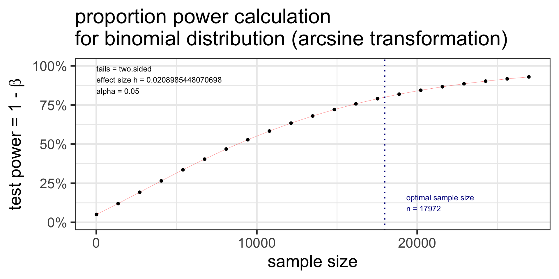
pwr: power for one proportion test

pwr.p.test(h = NULL, n = NULL, sig.level = 0.05, power = NULL,       alternative = c("two.sided","less","greater"))

• \(h\) is the effect size: h = ES.h(p1, p2)
  • p1 and p2 are the two proportions being tested
  • one of them is the null proportion \(p_0\), and the other is the alternative proportion

Specify all parameters except for the power:

library(pwr)

p.power <- pwr.p.test(
  h = ES.h(p1 = 0.36, p2 = 0.35),
  sig.level = 0.05, 
  # power = 0.80, 
  n = 269,
  alternative = "two.sided")
p.power

     proportion power calculation for binomial distribution (arcsine transformation) 

              h = 0.02089854
              n = 269
      sig.level = 0.05
          power = 0.06356445
    alternative = two.sided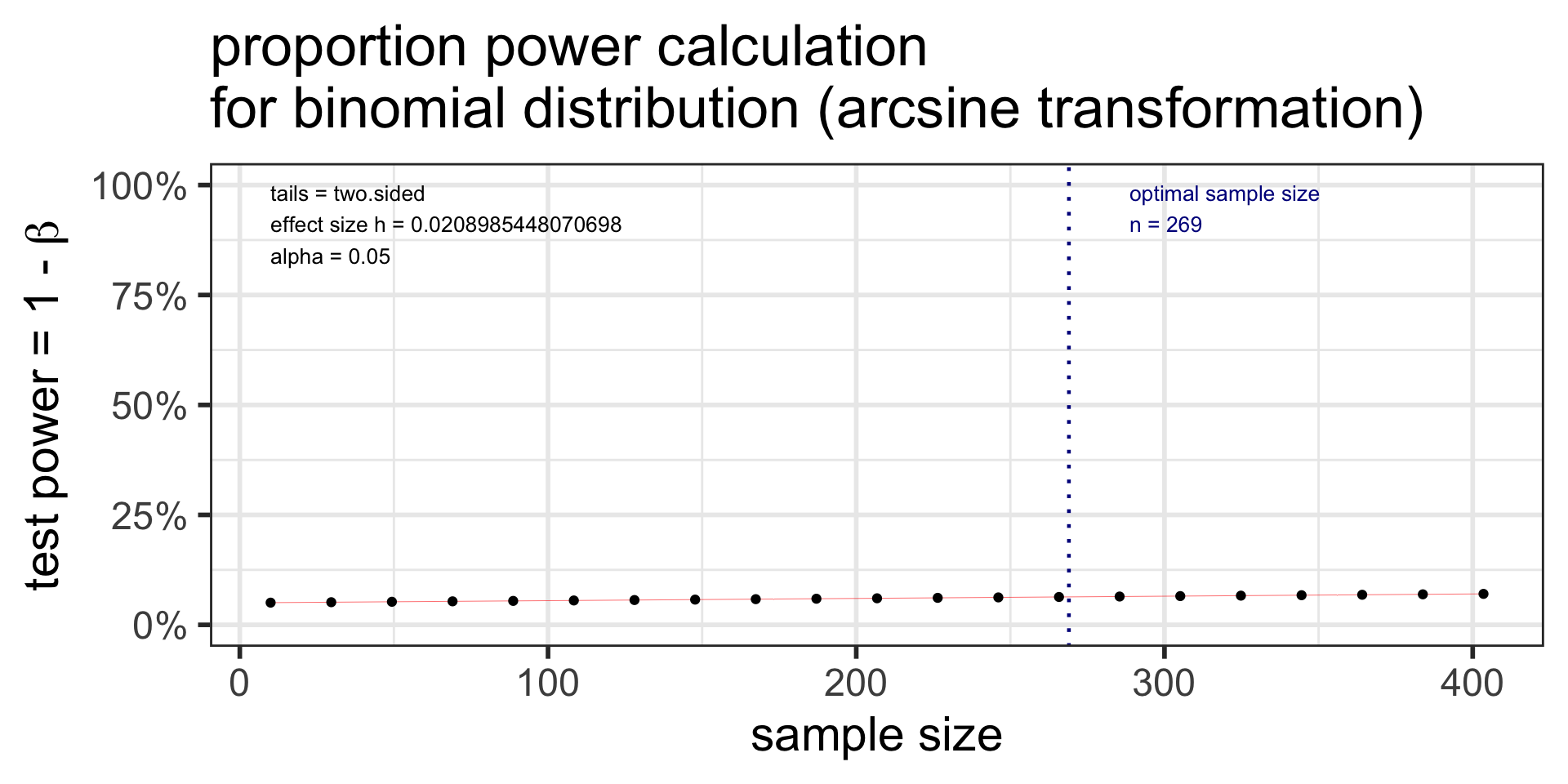

plot(p.power)

pwr: sample size for two proportions test

• Two proportions (same sample sizes)

pwr.2p.test(h = NULL, n = NULL, sig.level = 0.05, power = NULL,       alternative = c("two.sided","less","greater"))

• \(h\) is the effect size: h = ES.h(p1, p2); p1 and p2 are the two proportions being tested

Specify all parameters except for the sample size:

p2.n <- pwr.2p.test(
  h = ES.h(p1 = 0.36, p2 = 0.35),
  sig.level = 0.05, 
  power = 0.80, 
  alternative = "two.sided")
p2.n

     Difference of proportion power calculation for binomial distribution (arcsine transformation) 

              h = 0.02089854
              n = 35942.19
      sig.level = 0.05
          power = 0.8
    alternative = two.sided

NOTE: same sample sizes

Note: \(n\) in output is the number per sample!

plot(p2.n)

pwr: power for two proportions test

• Two proportions (different sample sizes)

pwr.2p2n.test(h = NULL, n1 = NULL, n2 = NULL, sig.level = 0.05, power = NULL,       alternative = c("two.sided", "less","greater"))

• \(h\) is the effect size: h = ES.h(p1, p2); p1 and p2 are the two proportions being tested

Specify all parameters except for the power:

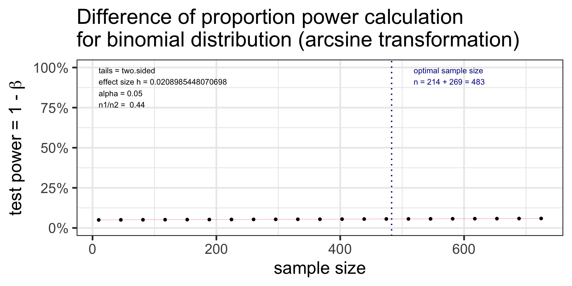
p2.n2 <- pwr.2p2n.test(
  h = ES.h(p1 = 0.36, p2 = 0.35),
  n1 = 214,
  n2 = 269,
  sig.level = 0.05, 
  # power = 0.80, 
  alternative = "two.sided")
p2.n2

     difference of proportion power calculation for binomial distribution (arcsine transformation) 

              h = 0.02089854
             n1 = 214
             n2 = 269
      sig.level = 0.05
          power = 0.05598413
    alternative = two.sided

NOTE: different sample sizes

Note: \(n\) in output is the number per sample!

plot(p2.n2)

Where are we?

CI’s and hypothesis tests for different scenarios:

\[\text{point estimate} \pm z^*(or~t^*)\cdot SE,~~\text{test stat} = \frac{\text{point estimate}-\text{null value}}{SE}\]

Day	Book	Population parameter	Symbol	Point estimate	Symbol	SE
10	5.1	Pop mean	\(\mu\)	Sample mean	\(\bar{x}\)	\(\frac{s}{\sqrt{n}}\)
10	5.2	Pop mean of paired diff	\(\mu_d\) or \(\delta\)	Sample mean of paired diff	\(\bar{x}_{d}\)	\(\frac{s_d}{\sqrt{n}}\)
11	5.3	Diff in pop means	\(\mu_1-\mu_2\)	Diff in sample means	\(\bar{x}_1 - \bar{x}_2\)	\(\sqrt{\frac{s_1^2}{n_1} + \frac{s_2^2}{n_2}}\) or pooled
12	8.1	Pop proportion	\(p\)	Sample prop	\(\widehat{p}\)	\(\sqrt{\frac{p(1-p)}{n}}\)
12	8.2	Diff in pop proportions	\(p_1-p_2\)	Diff in sample proportions	\(\widehat{p}_1-\widehat{p}_2\)	\(\sqrt{\frac{p_1\cdot(1-p_1)}{n_1} + \frac{p_2\cdot(1-p_2)}{n_2}}\)