Day 8: Variability in estimates

BSTA 511/611

Meike Niederhausen, PhD

OHSU-PSU School of Public Health

2024-10-28

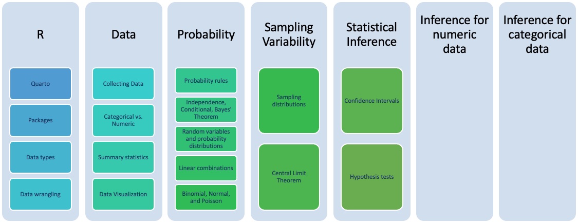
Where are we?

Goals for today

Section 4.1

• Sampling from a population
  • population parameters vs. point estimates
  • sampling variation
• Sampling distribution of the mean
  • Central Limit Theorem

Artwork by @allison_horst

MoRitz’s tip of the day: add a code pane in RStudio

Do you want to be able to view two code files side-by-side?
You can do that by adding a column to the RStudio layout.

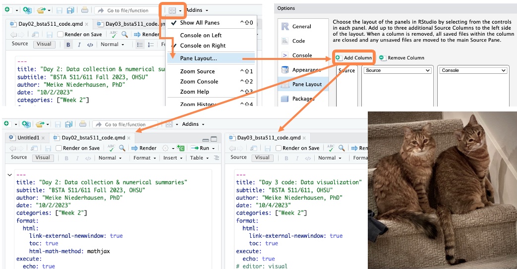
See https://posit.co/blog/rstudio-1-4-preview-multiple-source-columns/ for more information.

Population vs. sample (from section 1.3)

(Target) Population

• group of interest being studied
• group from which the sample is selected
  • studies often have inclusion and/or exclusion criteria

Sample

• group on which data are collected
• often a small subset of the population

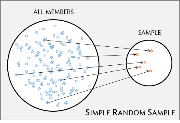
Simple random sample (SRS)

• each individual of a population has the same chance of being sampled
• randomly sampled
• considered best way to sample

Population parameters vs. sample statistics

Population parameter

Sample statistic (point estimate)

Our hypothetical population: YRBSS

Youth Risk Behavior Surveillance System (YRBSS)

• Yearly survey conducted by the US Centers for Disease Control (CDC)
• “A set of surveys that track behaviors that can lead to poor health in students grades 9 through 12.”¹
• Dataset yrbss from oibiostat pacakge contains responses from n = 13,583 participants in 2013 for a subset of the variables included in the complete survey data

library(oibiostat)
data("yrbss")  #load the data
# ?yrbss

dim(yrbss)

[1] 13583    13

names(yrbss)

 [1] "age"                      "gender"                  
 [3] "grade"                    "hispanic"                
 [5] "race"                     "height"                  
 [7] "weight"                   "helmet.12m"              
 [9] "text.while.driving.30d"   "physically.active.7d"    
[11] "hours.tv.per.school.day"  "strength.training.7d"    
[13] "school.night.hours.sleep"

1. Youth Risk Behavior Surveillance System https://www.cdc.gov/healthyyouth/data/yrbs/index.htm (YRBSS)

Getting to know the dataset: glimpse()

glimpse(yrbss)  # from tidyverse package (dplyr)

Rows: 13,583
Columns: 13
$ age                      <int> 14, 14, 15, 15, 15, 15, 15, 14, 15, 15, 15, 1…
$ gender                   <chr> "female", "female", "female", "female", "fema…
$ grade                    <chr> "9", "9", "9", "9", "9", "9", "9", "9", "9", …
$ hispanic                 <chr> "not", "not", "hispanic", "not", "not", "not"…
$ race                     <chr> "Black or African American", "Black or Africa…
$ height                   <dbl> NA, NA, 1.73, 1.60, 1.50, 1.57, 1.65, 1.88, 1…
$ weight                   <dbl> NA, NA, 84.37, 55.79, 46.72, 67.13, 131.54, 7…
$ helmet.12m               <chr> "never", "never", "never", "never", "did not …
$ text.while.driving.30d   <chr> "0", NA, "30", "0", "did not drive", "did not…
$ physically.active.7d     <int> 4, 2, 7, 0, 2, 1, 4, 4, 5, 0, 0, 0, 4, 7, 7, …
$ hours.tv.per.school.day  <chr> "5+", "5+", "5+", "2", "3", "5+", "5+", "5+",…
$ strength.training.7d     <int> 0, 0, 0, 0, 1, 0, 2, 0, 3, 0, 3, 0, 0, 7, 7, …
$ school.night.hours.sleep <chr> "8", "6", "<5", "6", "9", "8", "9", "6", "<5"…

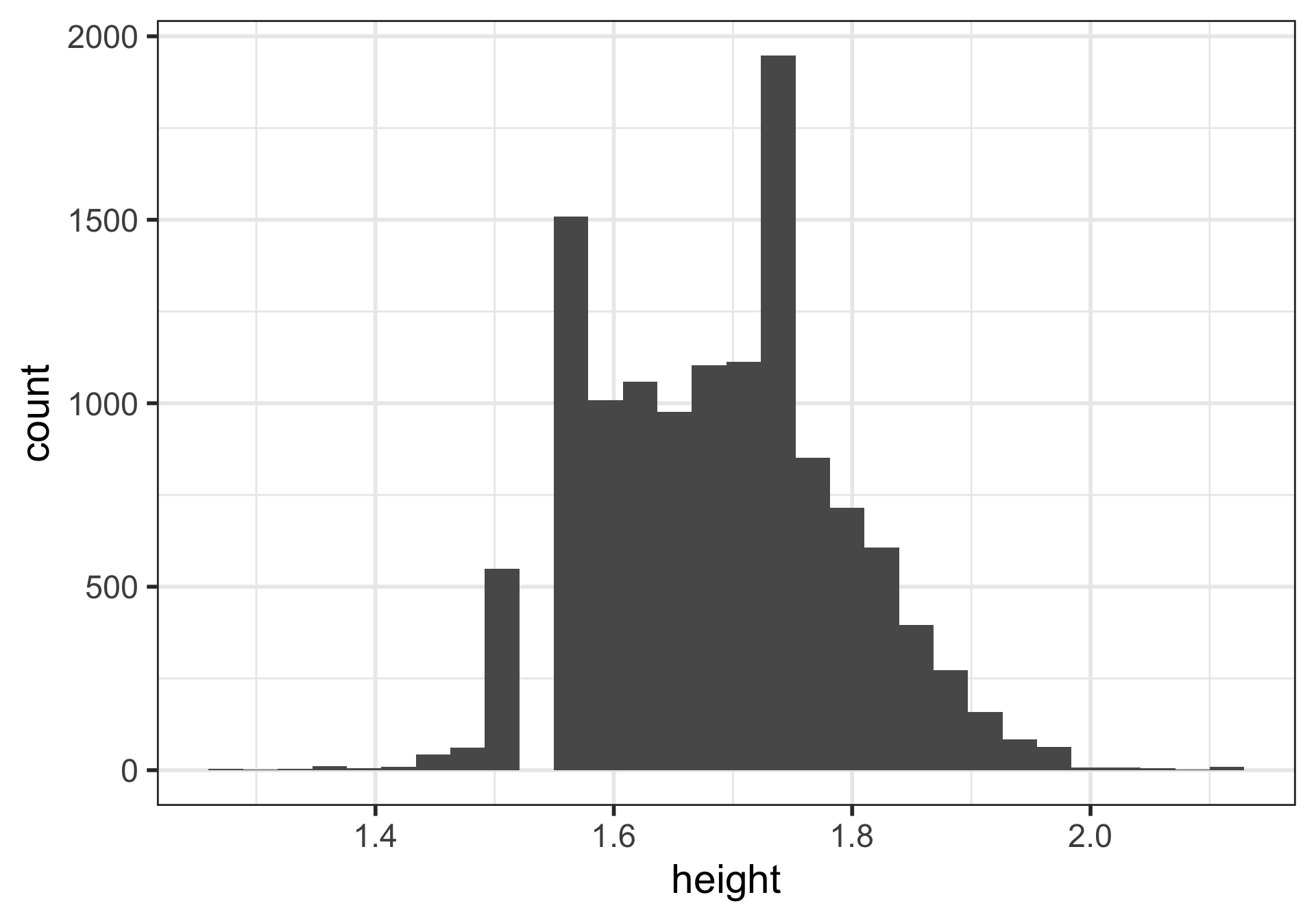
Height & weight variables

yrbss %>% 
  select(height, weight) %>% 
  summary()

     height          weight      
 Min.   :1.270   Min.   : 29.94  
 1st Qu.:1.600   1st Qu.: 56.25  
 Median :1.680   Median : 64.41  
 Mean   :1.691   Mean   : 67.91  
 3rd Qu.:1.780   3rd Qu.: 76.20  
 Max.   :2.110   Max.   :180.99  
 NA's   :1004    NA's   :1004    

ggplot(data = yrbss, 
       aes(x = height)) +
  geom_histogram()

Transform height & weight from metric to to standard

Also, drop missing values and add a column of id values

yrbss2 <- yrbss %>%                 # save new dataset with new name
  mutate(                           # add variables for 
    height.ft = 3.28084*height,     #     height in feet
    weight.lb = 2.20462*weight      #     weight in pounds
  ) %>% 
  drop_na(height.ft, weight.lb) %>% # drop rows w/ missing height/weight values
  mutate(id = 1:nrow(.)) %>%        # add id column
  select(id, height.ft, weight.lb)  # restrict dataset to columns of interest

head(yrbss2)  

  id height.ft weight.lb
1  1  5.675853  186.0038
2  2  5.249344  122.9957
3  3  4.921260  102.9998
4  4  5.150919  147.9961
5  5  5.413386  289.9957
6  6  6.167979  157.0130

dim(yrbss2)

[1] 12579     3

# number of rows deleted that had missing values for height and/or weight:
nrow(yrbss) - nrow(yrbss2) 

[1] 1004

yrbss2 summary

summary(yrbss2)

       id          height.ft       weight.lb     
 Min.   :    1   Min.   :4.167   Min.   : 66.01  
 1st Qu.: 3146   1st Qu.:5.249   1st Qu.:124.01  
 Median : 6290   Median :5.512   Median :142.00  
 Mean   : 6290   Mean   :5.549   Mean   :149.71  
 3rd Qu.: 9434   3rd Qu.:5.840   3rd Qu.:167.99  
 Max.   :12579   Max.   :6.923   Max.   :399.01  

Another summary:

yrbss2 %>% 
  get_summary_stats(type = "mean_sd") %>% 
  kable()

variable	n	mean	sd
id	12579	6290.000	3631.389
height.ft	12579	5.549	0.343
weight.lb	12579	149.708	37.254

Random sample of size n = 5 from yrbss2

Take a random sample of size n = 5 from yrbss2:

library(moderndive)
samp_n5_rep1 <- yrbss2 %>%
  rep_sample_n(size = 5, 
               reps = 1,
               replace = FALSE)
samp_n5_rep1

# A tibble: 5 × 4
# Groups:   replicate [1]
  replicate    id height.ft weight.lb
      <int> <int>     <dbl>     <dbl>
1         1  5869      5.15      145.
2         1  6694      5.41      127.
3         1  2517      5.74      130.
4         1  5372      6.07      180.
5         1  5403      6.07      163.

Calculate the mean of the random sample:

means_hght_samp_n5_rep1 <- 
  samp_n5_rep1 %>% 
  summarise(
    mean_height = mean(height.ft))

means_hght_samp_n5_rep1

# A tibble: 1 × 2
  replicate mean_height
      <int>       <dbl>
1         1        5.69

Would we get the same mean height if we took another sample?

Sampling variation

• If a different random sample is taken, the mean height (point estimate) will likely be different
  • this is a result of sampling variation

Take a 2nd random sample of size
n = 5 from yrbss2:

samp_n5_rep1 <- yrbss2 %>%
  rep_sample_n(size = 5, 
               reps = 1,
               replace = FALSE)
samp_n5_rep1

# A tibble: 5 × 4
# Groups:   replicate [1]
  replicate    id height.ft weight.lb
      <int> <int>     <dbl>     <dbl>
1         1  2329      6.07      182.
2         1  8863      5.25      125.
3         1  8058      5.84      135.
4         1   335      6.17      235.
5         1  4698      5.58      124.

Calculate the mean of the 2nd random sample:

means_hght_samp_n5_rep1 <- 
  samp_n5_rep1 %>% 
  summarise(
    mean_height = mean(height.ft))

means_hght_samp_n5_rep1

# A tibble: 1 × 2
  replicate mean_height
      <int>       <dbl>
1         1        5.78

Did we get the same mean height with our 2nd sample?

100 random samples of size n = 5 from yrbss2

Take 100 random samples of size
n = 5 from yrbss2:

samp_n5_rep100 <- yrbss2 %>%
  rep_sample_n(size = 5, 
               reps = 100,
               replace = FALSE)
samp_n5_rep100

# A tibble: 500 × 4
# Groups:   replicate [100]
   replicate    id height.ft weight.lb
       <int> <int>     <dbl>     <dbl>
 1         1  6483      5.51     145. 
 2         1  9899      4.92      90.0
 3         1  6103      5.68     118. 
 4         1  2702      5.68     150. 
 5         1 11789      5.35     115. 
 6         2 10164      5.51     140. 
 7         2  5807      5.41     215. 
 8         2  9382      5.15      98.0
 9         2  4904      6.00     196. 
10         2   229      6.07     101. 
# ℹ 490 more rows

Calculate the mean for each of the 100 random samples:

means_hght_samp_n5_rep100 <- 
  samp_n5_rep100 %>% 
  group_by(replicate) %>% 
  summarise(
    mean_height = mean(height.ft))

means_hght_samp_n5_rep100

# A tibble: 100 × 2
   replicate mean_height
       <int>       <dbl>
 1         1        5.43
 2         2        5.63
 3         3        5.34
 4         4        5.70
 5         5        5.90
 6         6        5.37
 7         7        5.49
 8         8        5.60
 9         9        5.50
10        10        5.68
# ℹ 90 more rows

How close are the mean heights for each of the 100 random samples?

Distribution of 100 sample mean heights (n = 5)

Describe the distribution shape.

ggplot(
  means_hght_samp_n5_rep100, 
  aes(x = mean_height)) + 
  geom_histogram()

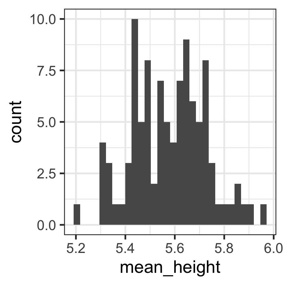
Calculate the mean and SD of the 100 mean heights from the 100 samples:

stats_means_hght_samp_n5_rep100 <- 
  means_hght_samp_n5_rep100 %>% 
  summarise(
   mean_mean_height = mean(mean_height),
   sd_mean_height = sd(mean_height)
   )
stats_means_hght_samp_n5_rep100

# A tibble: 1 × 2
  mean_mean_height sd_mean_height
             <dbl>          <dbl>
1             5.58          0.150

Is the mean of the means close to the “center” of the distribution?

10,000 random samples of size n = 5 from yrbss2

Take 10,000 random samples of size
n = 5 from yrbss2:

samp_n5_rep10000 <- yrbss2 %>%
  rep_sample_n(size = 5, 
               reps = 10000,
               replace = FALSE)
samp_n5_rep10000

# A tibble: 50,000 × 4
# Groups:   replicate [10,000]
   replicate    id height.ft weight.lb
       <int> <int>     <dbl>     <dbl>
 1         1  6383      5.35      126.
 2         1  4019      5.41      107.
 3         1  4856      5.25      135.
 4         1  9988      5.58      120.
 5         1  2245      6.17      270.
 6         2 10580      5.68      155.
 7         2  2254      5.84      159.
 8         2  8081      5.09      110.
 9         2 10194      5.35      115.
10         2  7689      5.35      135.
# ℹ 49,990 more rows

Calculate the mean for each of the 10,000 random samples:

means_hght_samp_n5_rep10000 <- 
  samp_n5_rep10000 %>% 
  group_by(replicate) %>% 
  summarise(
    mean_height = mean(height.ft))

means_hght_samp_n5_rep10000

# A tibble: 10,000 × 2
   replicate mean_height
       <int>       <dbl>
 1         1        5.55
 2         2        5.46
 3         3        5.49
 4         4        5.60
 5         5        5.47
 6         6        5.83
 7         7        5.68
 8         8        5.47
 9         9        5.37
10        10        5.15
# ℹ 9,990 more rows

How close are the mean heights for each of the 10,000 random samples?

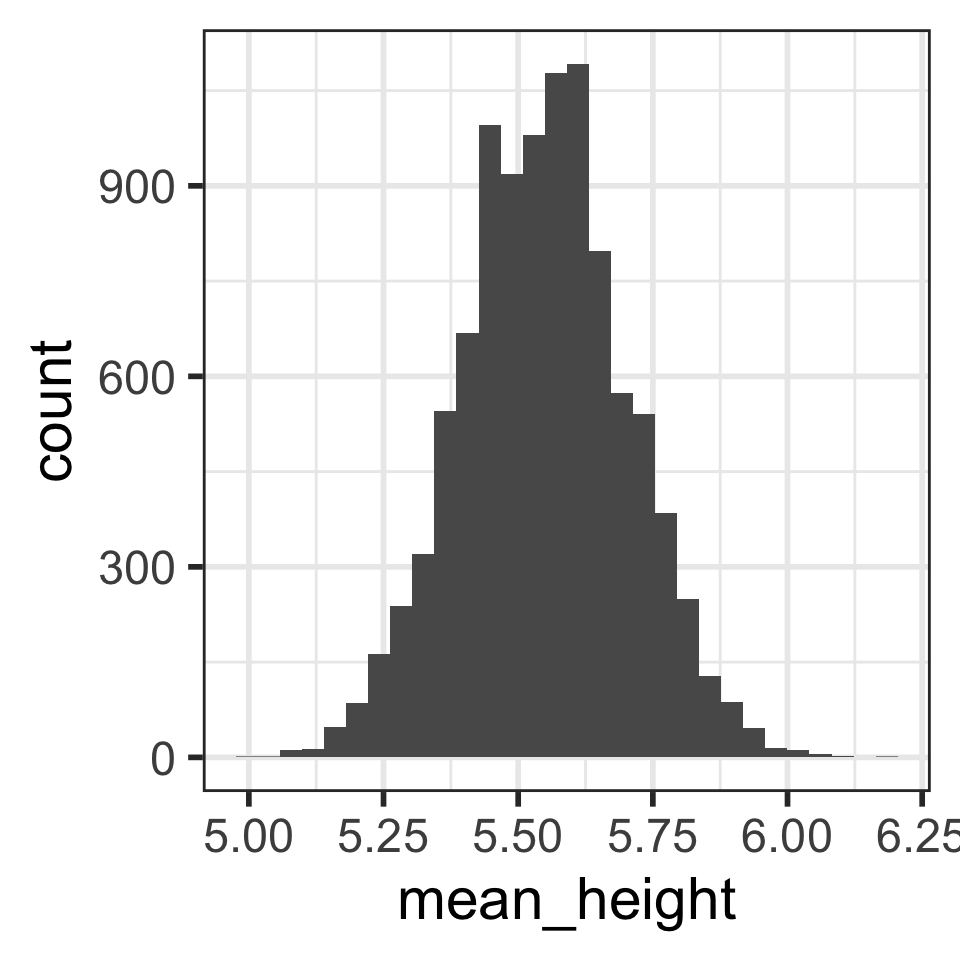
Distribution of 10,000 sample mean heights (n = 5)

Describe the distribution shape.

ggplot(
  means_hght_samp_n5_rep10000, 
  aes(x = mean_height)) + 
  geom_histogram()

Calculate the mean and SD of the 10,000 mean heights from the 10,000 samples:

stats_means_hght_samp_n5_rep10000 <- 
  means_hght_samp_n5_rep10000 %>% 
  summarise(
   mean_mean_height=mean(mean_height),
   sd_mean_height = sd(mean_height)
   )
stats_means_hght_samp_n5_rep10000

# A tibble: 1 × 2
  mean_mean_height sd_mean_height
             <dbl>          <dbl>
1             5.55          0.153

Is the mean of the means close to the “center” of the distribution?

10,000 samples of size n = 30 from yrbss2

Take 10,000 random samples of size
n = 30 from yrbss2:

samp_n30_rep10000 <- yrbss2 %>%
  rep_sample_n(size = 30, 
               reps = 10000,
               replace = FALSE)
samp_n30_rep10000

# A tibble: 300,000 × 4
# Groups:   replicate [10,000]
   replicate    id height.ft weight.lb
       <int> <int>     <dbl>     <dbl>
 1         1  3871      5.25      115.
 2         1 12090      5.15      125.
 3         1   241      5.58      119.
 4         1  4570      5.58      140.
 5         1  4131      5.35      143.
 6         1 11513      5.35      135.
 7         1  9663      5.25      125.
 8         1  3789      5.25      160.
 9         1   442      5.15      130.
10         1 11528      5.51      200.
# ℹ 299,990 more rows

Calculate the mean for each of the 10,000 random samples:

means_hght_samp_n30_rep10000 <- 
  samp_n30_rep10000 %>% 
  group_by(replicate) %>% 
  summarise(mean_height = 
            mean(height.ft))

means_hght_samp_n30_rep10000

# A tibble: 10,000 × 2
   replicate mean_height
       <int>       <dbl>
 1         1        5.48
 2         2        5.63
 3         3        5.46
 4         4        5.46
 5         5        5.51
 6         6        5.54
 7         7        5.56
 8         8        5.51
 9         9        5.51
10        10        5.50
# ℹ 9,990 more rows

How close are the mean heights for each of the 10,000 random samples?

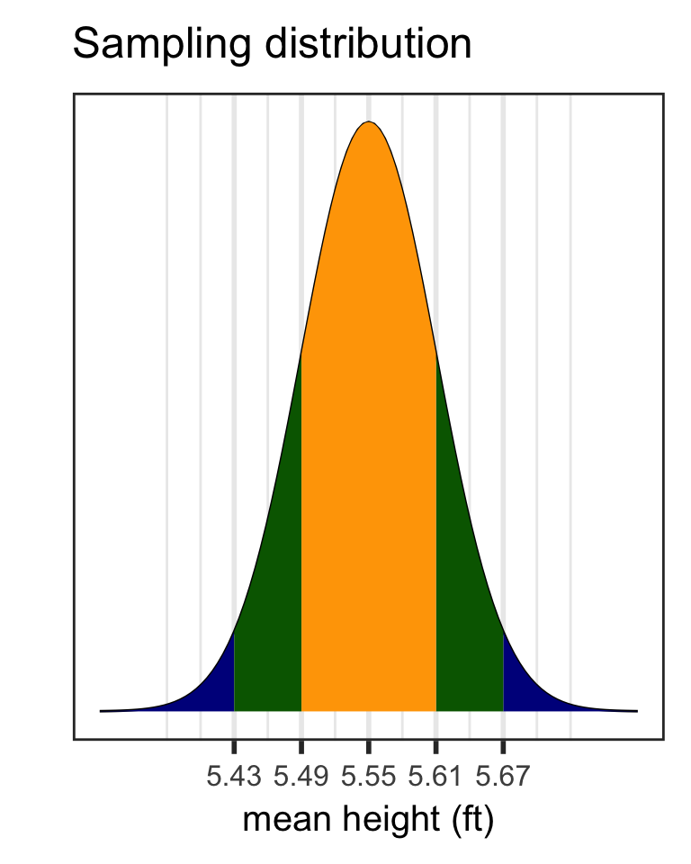
Distribution of 10,000 sample mean heights (n = 30)

Describe the distribution shape.

ggplot(
  means_hght_samp_n30_rep10000, 
  aes(x = mean_height)) + 
  geom_histogram()

Calculate the mean and SD of the 10,000 mean heights from the 10,000 samples:

stats_means_hght_samp_n30_rep10000<- 
  means_hght_samp_n30_rep10000 %>% 
  summarise(
   mean_mean_height=mean(mean_height),
   sd_mean_height = sd(mean_height)
   )
stats_means_hght_samp_n30_rep10000

# A tibble: 1 × 2
  mean_mean_height sd_mean_height
             <dbl>          <dbl>
1             5.55         0.0623

Is the mean of the means close to the “center” of the distribution?

Compare distributions of 10,000 sample mean heights when n = 5 (left) vs. n = 30 (right)

How are the center, shape, and spread similar and/or different?

# A tibble: 1 × 2
  mean_mean_height sd_mean_height
             <dbl>          <dbl>
1             5.55          0.153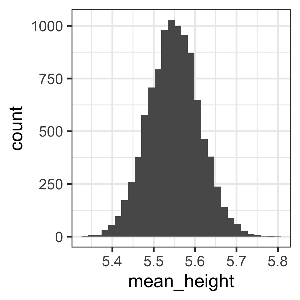

# A tibble: 1 × 2
  mean_mean_height sd_mean_height
             <dbl>          <dbl>
1             5.55         0.0623

Sampling high schoolers’ weights

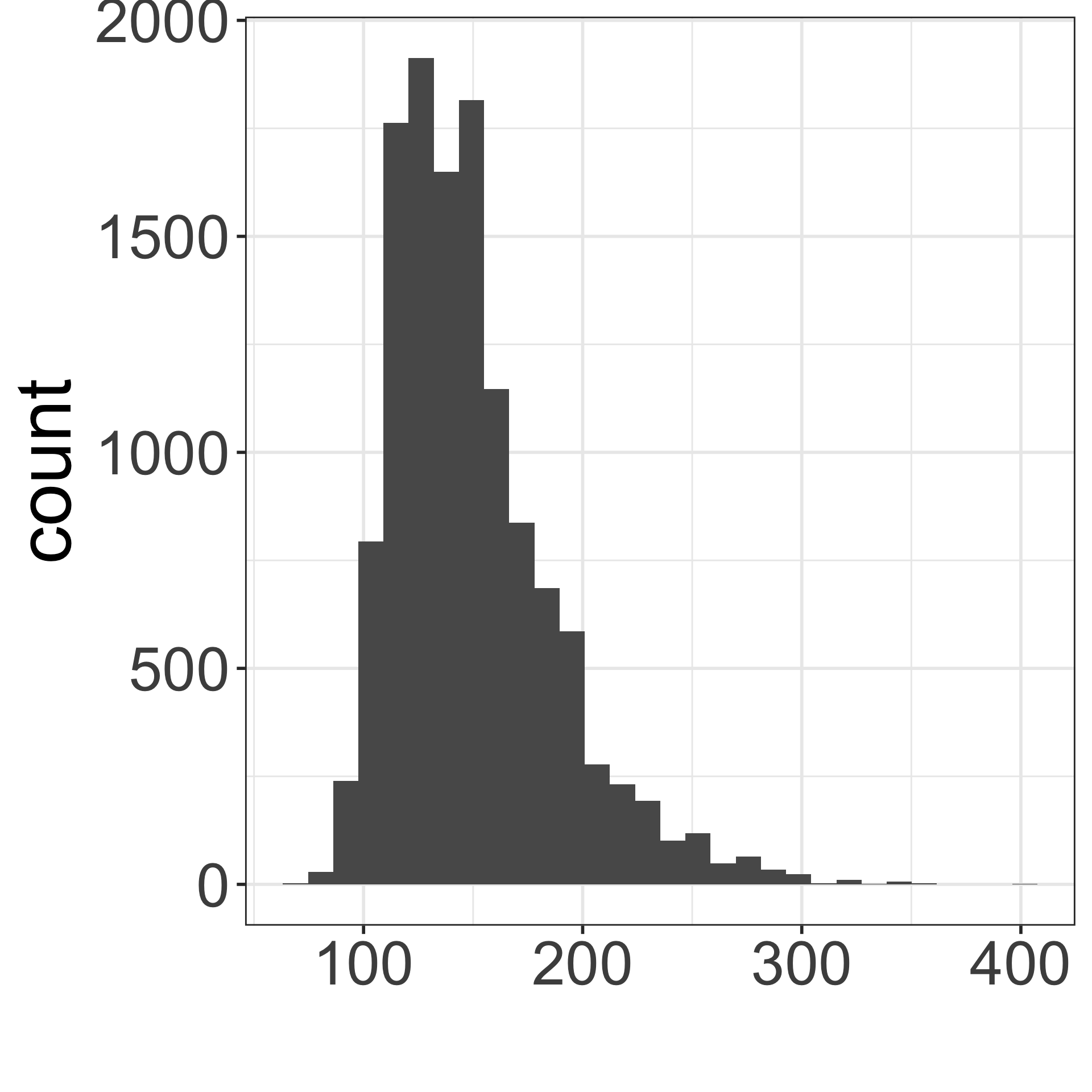
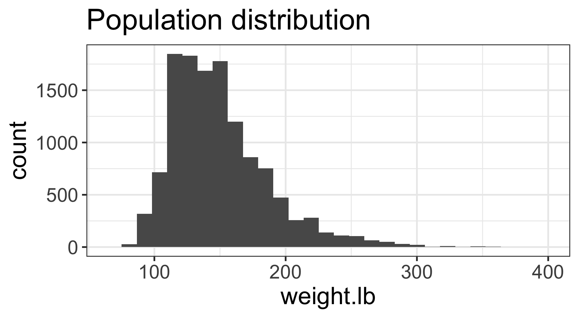
Which figure is which?

• Population distribution of weights
• Sampling distribution of mean weights when \(n=5\)
• Sampling distribution of mean weights when \(n=30\).

A

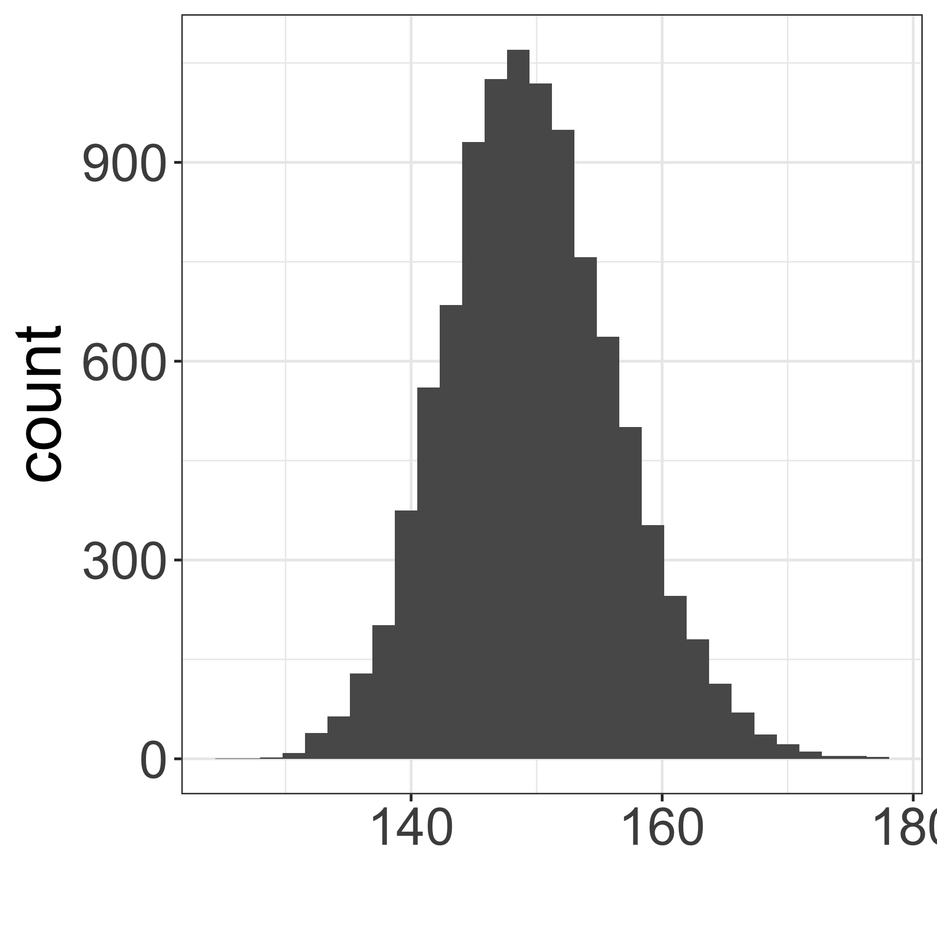
B

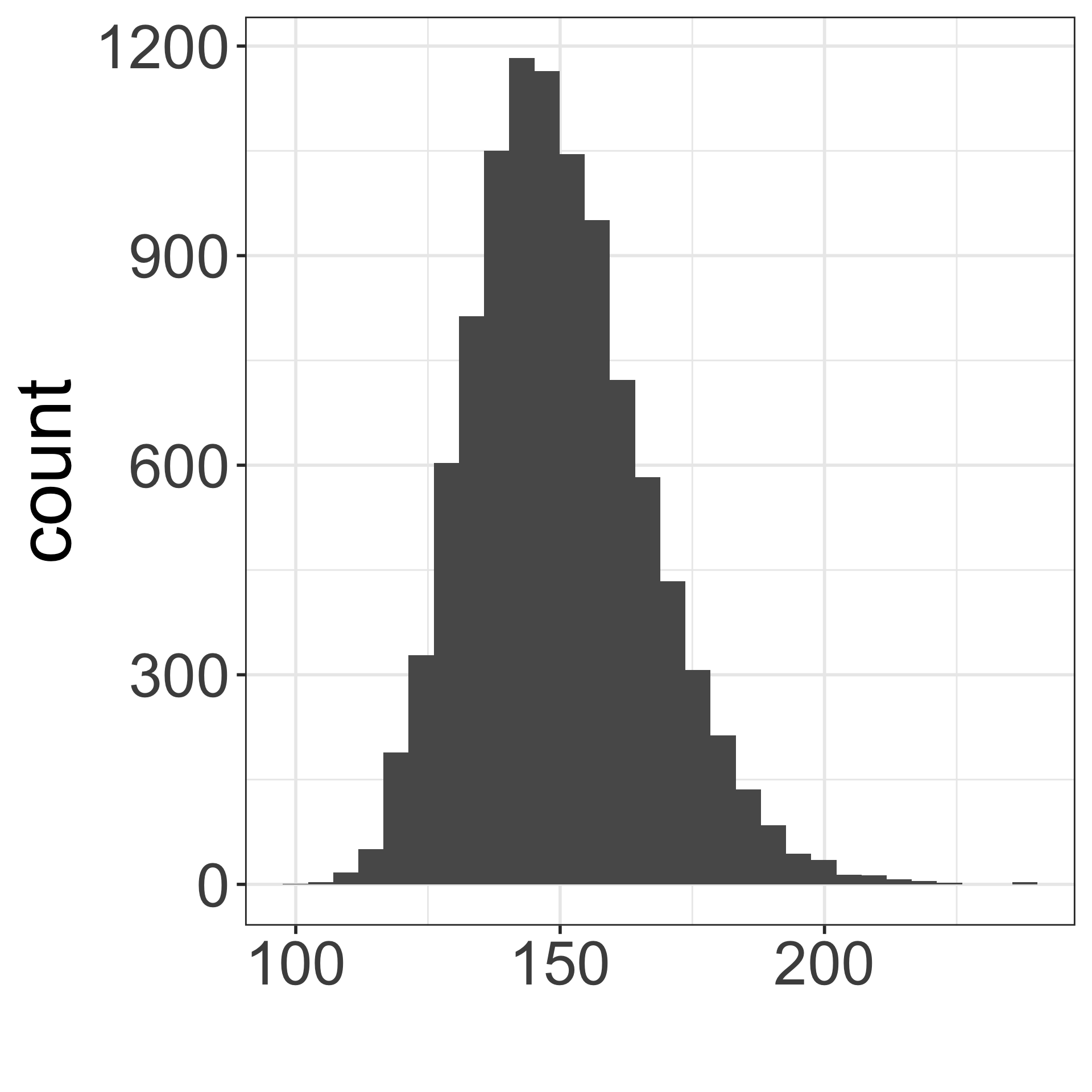
C

The sampling distribution of the mean

• The sampling distribution of the mean is the distribution of sample means calculated from repeated random samples of the same size from the same population

• Our simulations show approximations of the sampling distribution of the mean for various sample sizes

• The theoretical sampling distribution is based on all possible samples of a given sample size \(n\).

The Central Limit Theorem (CLT)

• For “large” sample sizes ( \(n\geq 30\) ),
  • the sampling distribution of the sample mean
  • can be approximated by a normal distribution,with
    • mean equal to the population mean value \(\mu\), and
    • standard deviation \(\frac{\sigma}{\sqrt{n}}\)

• For small sample sizes, if the population is known to be normally distributed, then
  • the sampling distribution of the sample mean
  • is a normal distribution, with
    • mean equal to the population mean value \(\mu\), and
    • standard deviation \(\frac{\sigma}{\sqrt{n}}\)

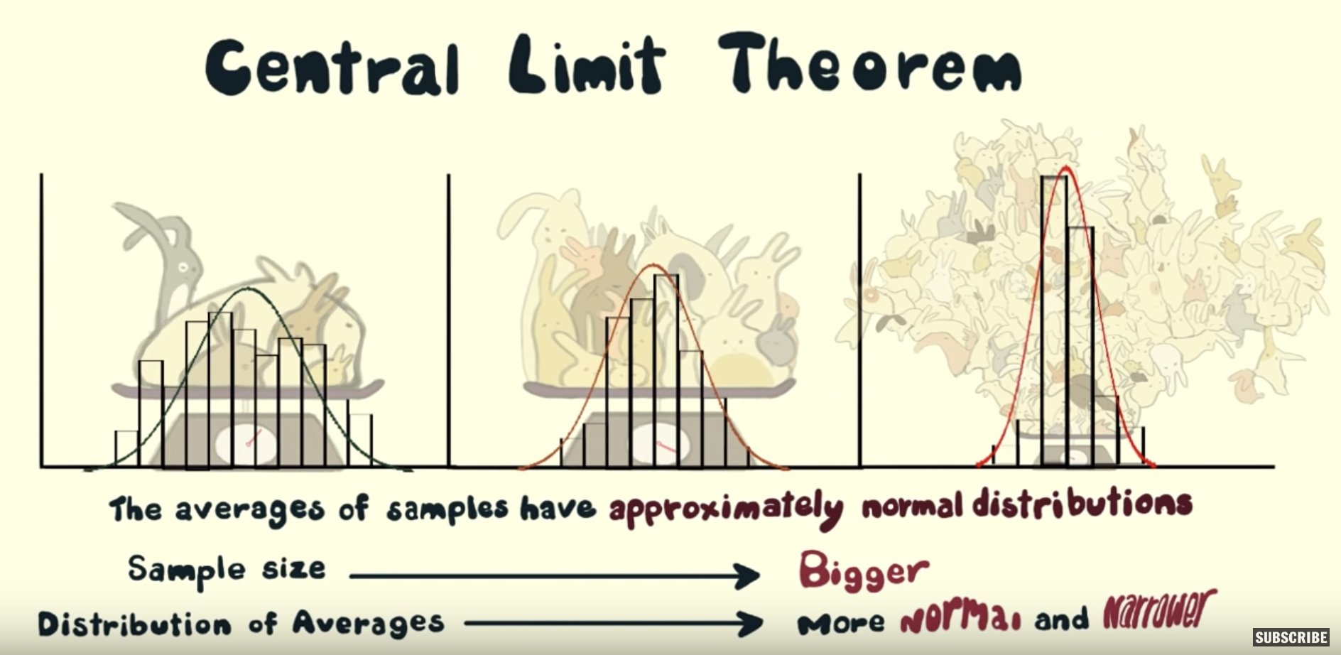
The cutest statistics video on YouTube

• Bunnies, Dragons and the ‘Normal’ World: Central Limit Theorem
  • Creature Cast from the New York Times
  • https://www.youtube.com/watch?v=jvoxEYmQHNM&feature=youtu.be

Sampling distribution of mean heights when n = 30 (1/2)

ggplot(
  means_hght_samp_n30_rep10000, 
  aes(x = mean_height)) + 
  geom_histogram()

CLT tells us that we can model the sampling distribution of mean heights using a normal distribution.

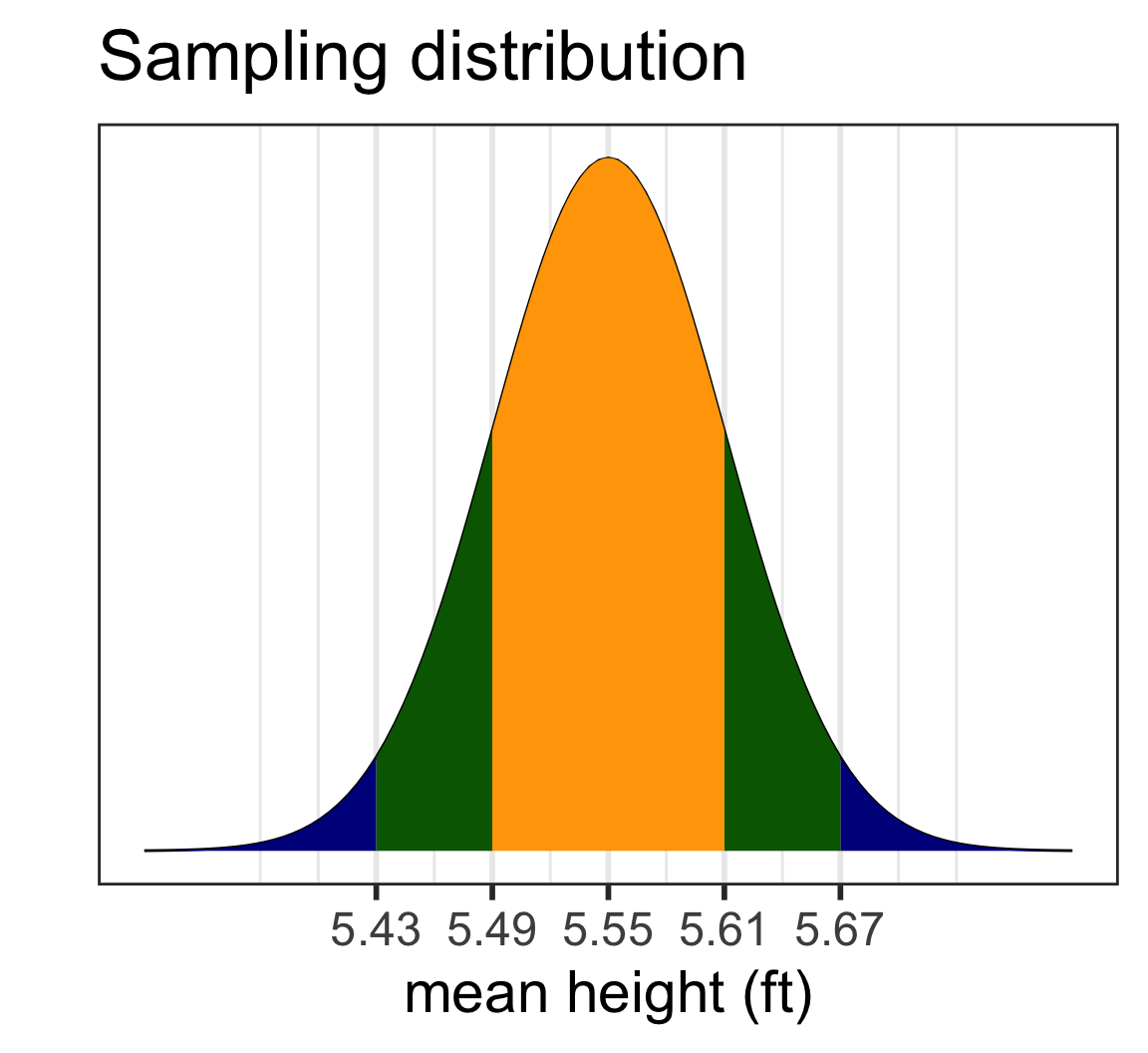
Sampling distribution of mean heights when n = 30 (2/2)

Mean and SD of population:

(mean_height.ft <- mean(yrbss2$height.ft))

[1] 5.548691

(sd_height.ft <- sd(yrbss2$height.ft))

[1] 0.3434949

sd_height.ft/sqrt(30)

[1] 0.06271331

Mean and SD of simulated sampling distribution:

stats_means_hght_samp_n30_rep10000<- 
  means_hght_samp_n30_rep10000 %>% 
  summarise(
   mean_mean_height=mean(mean_height),
   sd_mean_height = sd(mean_height)
   )
stats_means_hght_samp_n30_rep10000

# A tibble: 1 × 2
  mean_mean_height sd_mean_height
             <dbl>          <dbl>
1             5.55         0.0623

Why is the mean \(\mu\) & the standard error \(\frac{\sigma}{\sqrt{n}}\) ?

Applying the CLT

What is the probability that for a random sample of 30 high schoolers, that their mean height is greater than 5.6 ft?

Class Discussion

• Slide 21: match figures to distribution (Sampling high schoolers’ weights)

Problems from Homework 4:

• R1: Youth weights (YRBSS)
• Book exercise: 4.2
• Non-book exercise: Ethan Allen