Day 3: Data visualization - Part 2
BSTA 511/611 Fall 2024 Day 5, OHSU
2024-10-16
Recall previous data viz
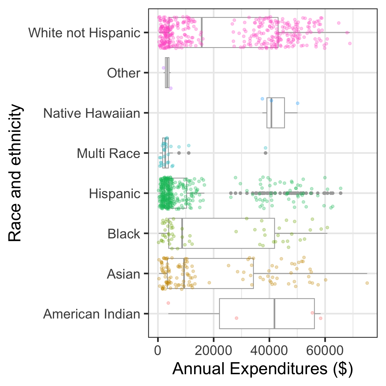
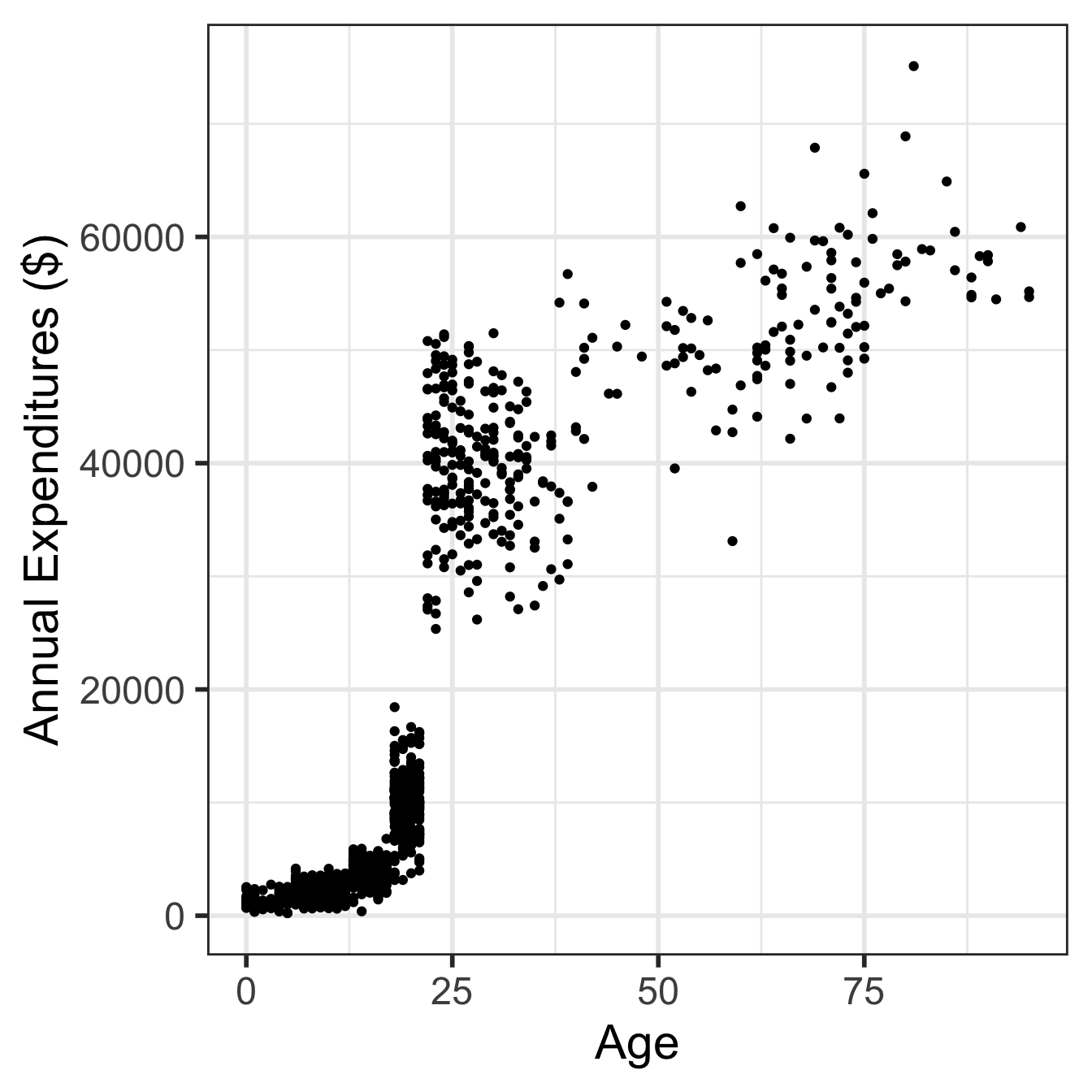
Visualize in more detail:
ethnicity, age, and expenditures (code on next slide)
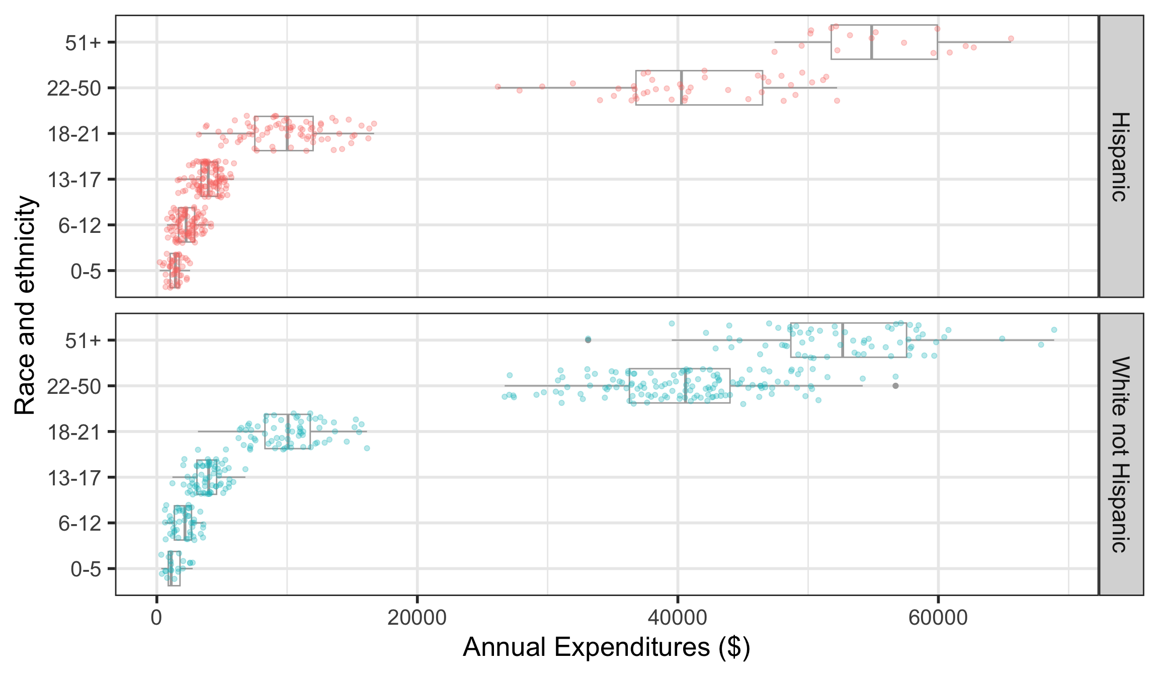
Simpson’s paradox
This case study is an example of confounding known as Simpson’s paradox
Simpson’s paradox happens when an association observed in several groups disappears or reverses direction when the groups are combined.
In other words, an association between two variables \(X\) and \(Y\) may disappear or reverse direction once data are partitioned into subpopulations based on a third variable \(Z\) (i.e., a confounding variable).

The tidyverse

What packages are included in the tidyverse?
Core packages
These automatically load when loading the tidyverse package

List of all packages:
 [1] "broom"         "conflicted"    "cli"           "dbplyr"
 [5] "dplyr"         "dtplyr"        "forcats"       "ggplot2"
 [9] "googledrive"   "googlesheets4" "haven"         "hms"
[13] "httr"          "jsonlite"      "lubridate"     "magrittr"
[17] "modelr"        "pillar"        "purrr"         "ragg"
[21] "readr"         "readxl"        "reprex"        "rlang"
[25] "rstudioapi"    "rvest"         "stringr"       "tibble"
[29] "tidyr" "xml2" "tidyverse" - Packages not a part of the core get installed with the tidyverse suite, but need to be loaded separately.
- See https://www.tidyverse.org/packages/ for more info.