Yearly survey conducted by the US Centers for Disease Control (CDC)
“A set of surveys that track behaviors that can lead to poor health in students grades 9 through 12.”1
Dataset yrbss from oibiostat pacakge contains responses from n = 13,583 participants in 2013 for a subset of the variables included in the complete survey data
library(oibiostat)data("yrbss") #load the data# ?yrbss
Transform height & weight from metric to to standard
Also, drop missing values and add a column of id values
yrbss2 <- yrbss %>%# save new dataset with new namemutate( # add variables for height.ft =3.28084*height, # height in feetweight.lb =2.20462*weight # weight in pounds ) %>%drop_na(height.ft, weight.lb) %>%# drop rows w/ missing height/weight valuesmutate(id =1:nrow(.)) %>%# add id columnselect(id, height.ft, weight.lb) # restrict dataset to columns of interesthead(yrbss2)
# number of rows deleted that had missing values for height and/or weight:nrow(yrbss) -nrow(yrbss2)
[1] 1004
yrbss2: stats for height in feet
summary(yrbss2)
       id          height.ft       weight.lb
 Min.   :    1   Min.   :4.167   Min.   : 66.01
 1st Qu.: 3146   1st Qu.:5.249   1st Qu.:124.01
 Median : 6290   Median :5.512   Median :142.00
 Mean   : 6290   Mean   :5.549   Mean   :149.71
 3rd Qu.: 9434   3rd Qu.:5.840   3rd Qu.:167.99
 Max.   :12579   Max.   :6.923   Max.   :399.01
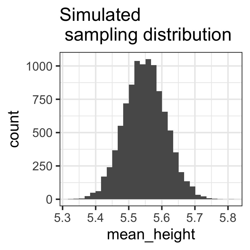
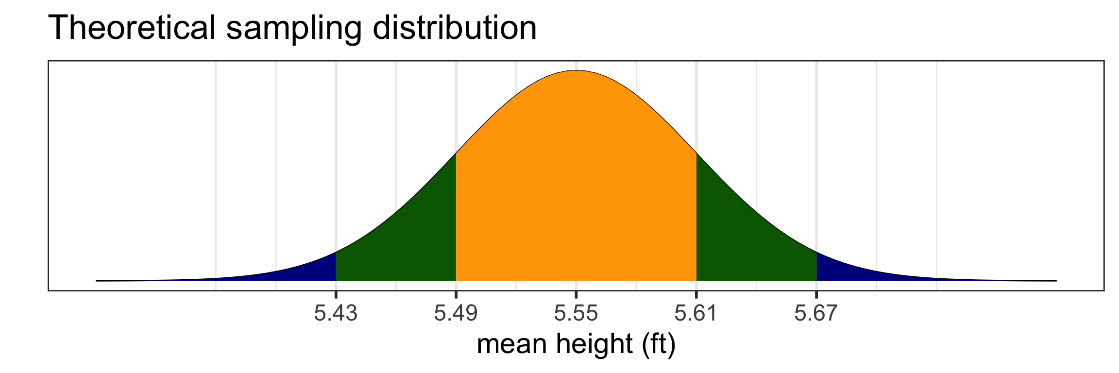
(mean_height.ft <-mean(yrbss2$height.ft))
[1] 5.548691
(sd_height.ft <-sd(yrbss2$height.ft))
[1] 0.3434949
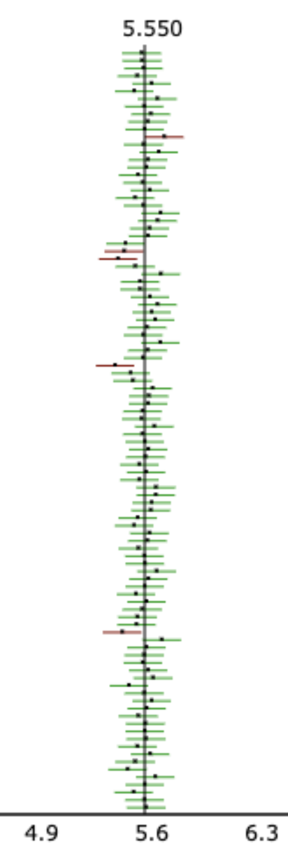
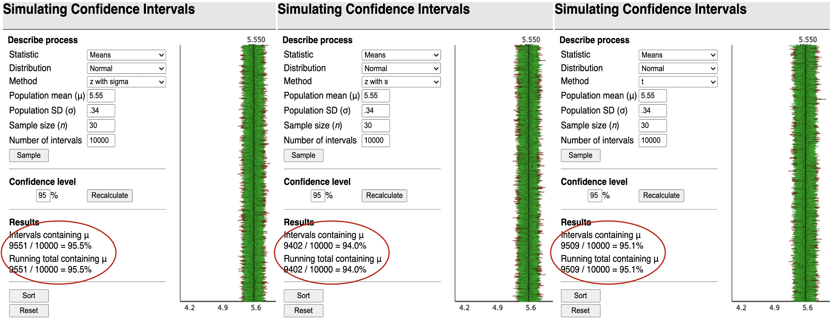
10,000 samples of size n = 30 from yrbss2
Take 10,000 random samples of size
n = 30 from yrbss2:
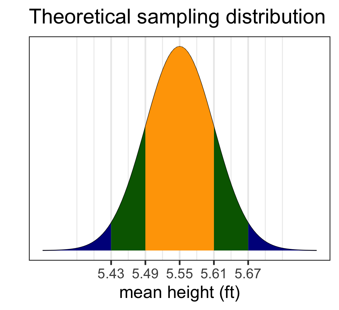
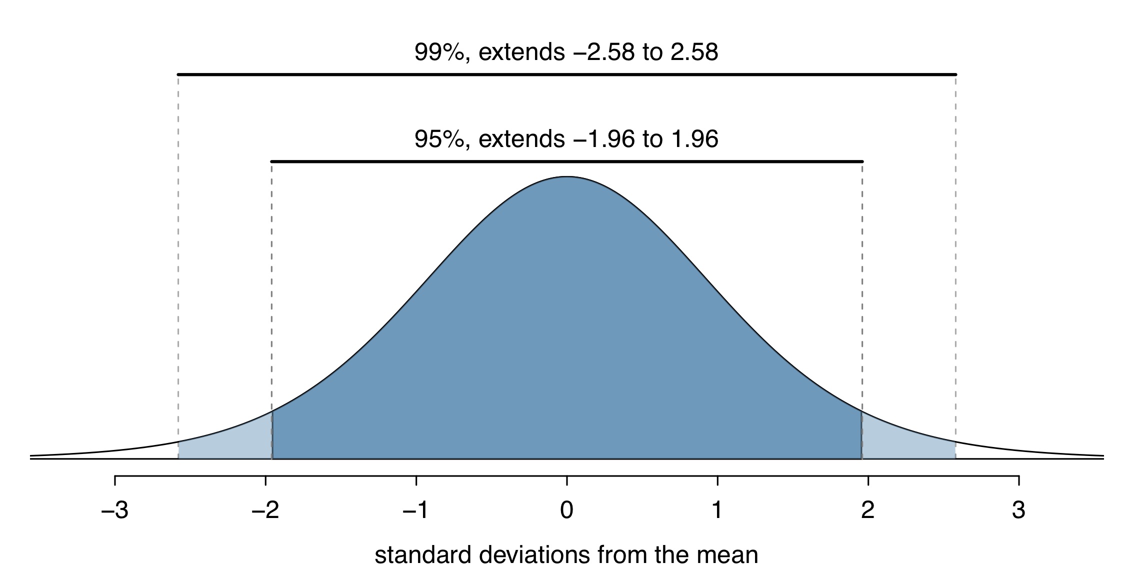
The normal distribution doesn’t have a 95% “coverage rate”
when using \(s\) instead of \(\sigma\)
What if we don’t know \(\sigma\) ? (2/3)
In real life, we don’t know what the population sd is ( \(\sigma\) )
If we replace \(\sigma\) with \(s\) in the SE formula, we add in additional variability to the SE! \[\frac{\sigma}{\sqrt{n}} ~~~~\textrm{vs.} ~~~~ \frac{s}{\sqrt{n}}\]
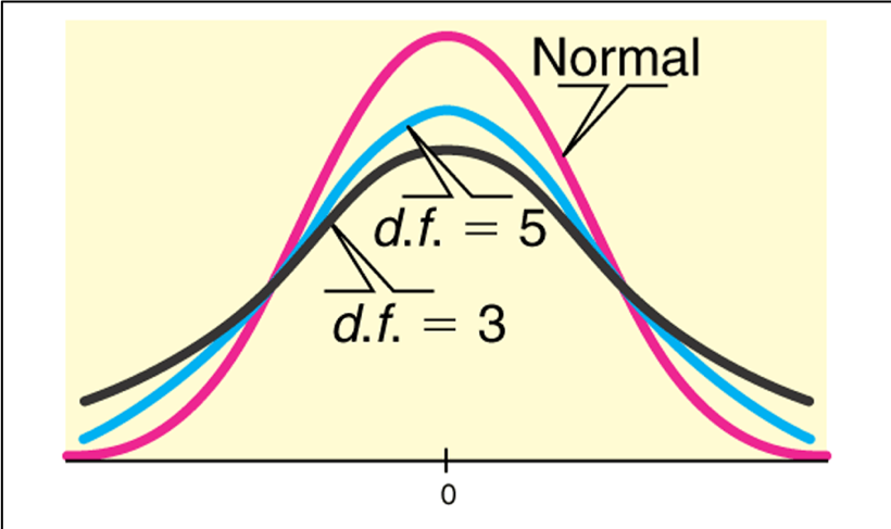
Thus when using \(s\) instead of \(\sigma\) when calculating the SE, we need a different probability distribution with thicker tails than the normal distribution.
In practice this will mean using a different value than 1.96 when calculating the CI.
What if we don’t know \(\sigma\) ? (3/3)
The Student’s t-distribution:
Is bell shaped and symmetric with mean = 0.
Its tails are a thicker than that of a normal distribution
The “thickness” depends on its degrees of freedom: \(df = n–1\) , where n = sample size.
As the degrees of freedom (sample size) increase,
the tails are less thick, and
the t-distribution is more like a normal distribution
in theory, with an infinite sample size the t-distribution is a normal distribution.
Calculating the C I for the population mean using \(s\)
CI for \(\mu\):
\[\bar{x} \pm t^*\cdot\frac{s}{\sqrt{n}}\]
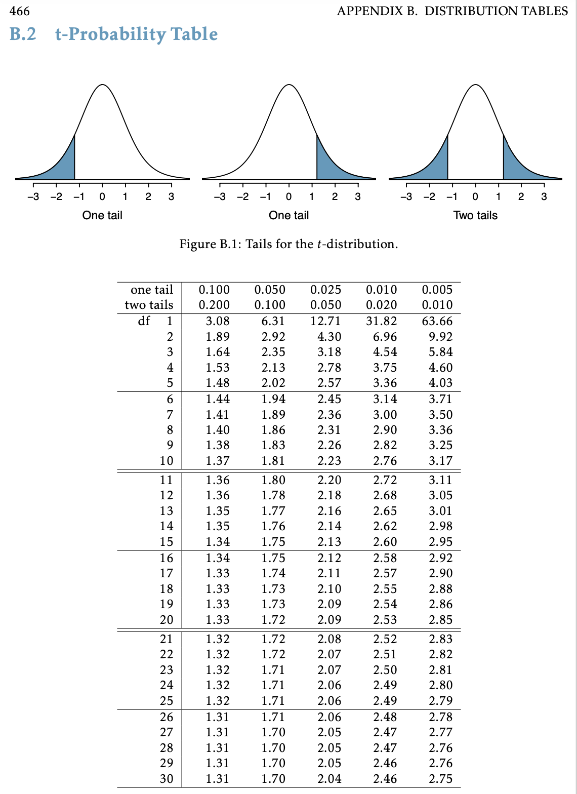
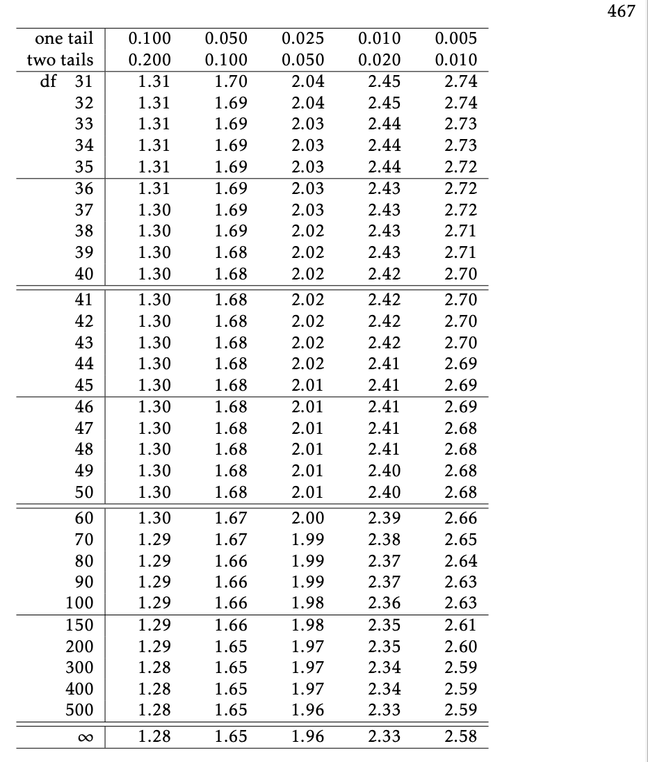
where \(t^*\) is determined by the t-distribution and dependent on the df =\(n-1\) and the confidence level
qt gives the quartiles for a t-distribution. Need to specify
the percent under the curve to the left of the quartile
the degrees of freedom = n-1
Note in the R output to the right that \(t^*\) gets closer to 1.96 as the sample size increases.
qt(.975, df=9) # df = n-1
[1] 2.262157
qt(.975, df=49)
[1] 2.009575
qt(.975, df=99)
[1] 1.984217
qt(.975, df=999)
[1] 1.962341
Using a \(t\)-table to get \(t^*\)
Example: C I for mean height (revisited)
A random sample of 30 high schoolers has mean height 5.6 ft and standard deviation 0.34 ft.
Find the 95% confidence interval for the population mean.
\(z\) vs \(t\)?? (& important comment about Chapter 4 of textbook)
Textbook’s rule of thumb
(Ch 4) If \(n \geq 30\) and population distribution not strongly skewed:
Use normal distribution
No matter if using \(\sigma\) or \(s\) for the \(SE\)
If there is skew or some large outliers, then need \(n \geq 50\)
(Ch 5) If \(n < 30\) and data approximately symmetric with no large outliers:
Use Student’s t-distribution
BSTA 511 rule of thumb
Use normal distribution ONLY if know \(\sigma\)
If using \(s\) for the \(SE\), then use the Student’s t-distribution
For either case, can apply if either
\(n \geq 30\) and population distribution not strongly skewed
If there is skew or some large outliers, then \(n \geq 50\) gives better estimates
\(n < 30\) and data approximately symmetric with no large outliers
If do not know population distribution, then check the distribution of the data.